Expectations for Statistical Arbitrage in Energy Futures Markets

1
The Kansai Electric Power Company, Incorporated, 6-16, Nakanoshima 3-chome, Kita-Ku, Osaka 530-8270, Japan
2
Graduate School of Economics, Kobe University, 2-1 Rokkodai-cho Nada-ku, Kobe 657-8501, Japan
J. Risk Financial Manag. 2019, 12(1), 14; https://doi.org/10.3390/jrfm12010014
Submission received: 7 December 2018
/
Revised: 8 January 2019
/
Accepted: 12 January 2019
/
Published: 15 January 2019
(This article belongs to the Special Issue Energy Finance and Sustainable Development)
Abstract
:Energy futures have become important as alternative investment assets to minimize the volatility of portfolio return, owing to their low links with traditional financial markets. In order to make energy futures markets grow further, it is necessary to expand expectations of returns from trading in energy futures markets. Therefore, this study examines whether profits can be earned by statistical arbitrage between wholesale electricity futures and natural gas futures listed on the New York Mercantile Exchange. On the assumption that power prices and natural gas prices have a cointegration relationship, as tested and supported by previous studies, the short-term deviation from the long-term equilibrium is regarded as an arbitrage opportunity. The results of the spark-spread trading simulations using historical data from 2 January 2014 to 29 December 2017 show about 30% yield at maximum. This study shows the possibility of generating earnings in energy futures market.
1. Introduction
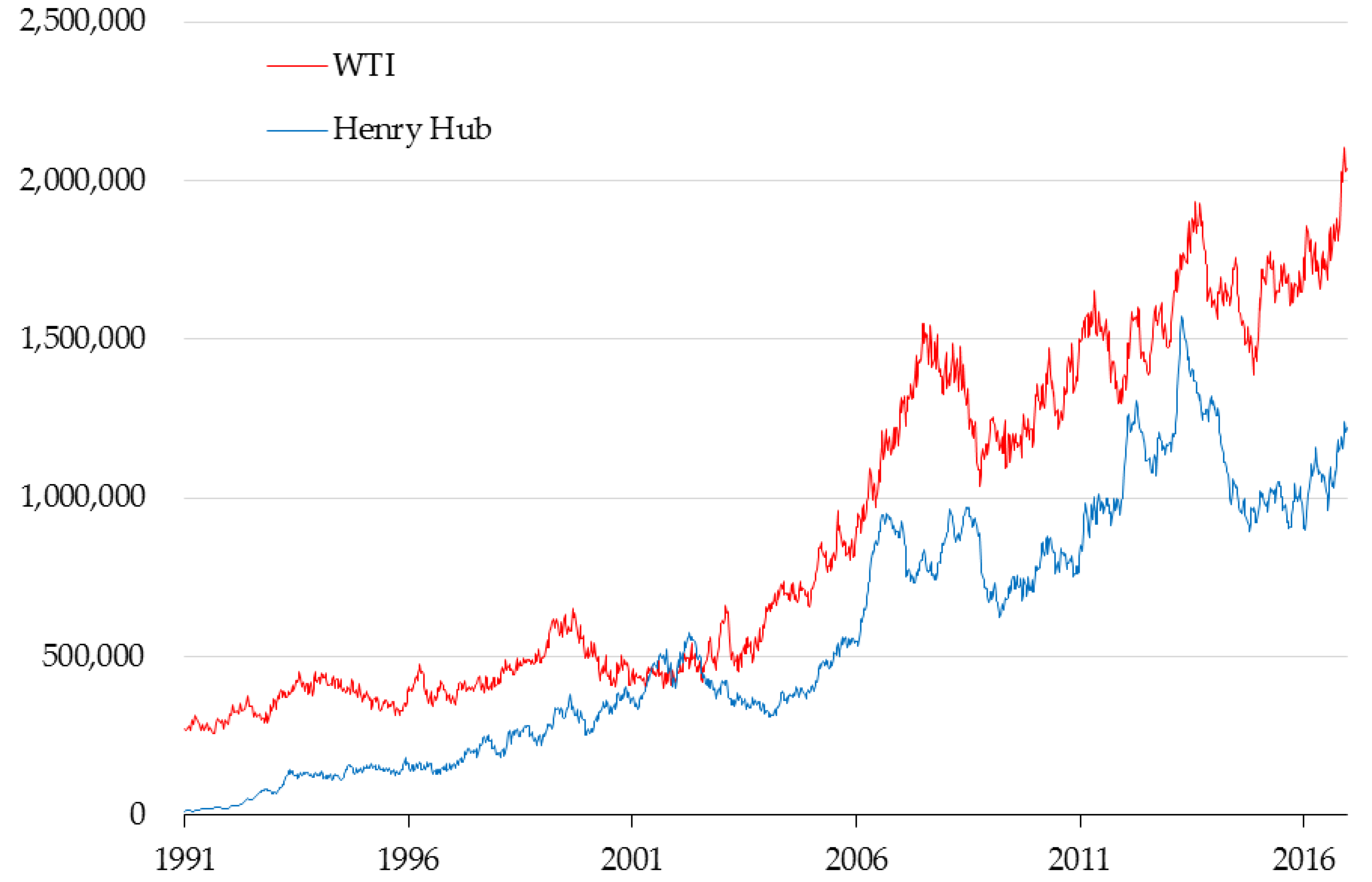
A variety of energy derivatives are listed and actively traded on the New York Mercantile Exchange (NYMEX), the Intercontinental Exchange Futures, and other commodity exchanges. For example, Figure 1 traces the open interests of West Texas Intermediate (WTI) crude oil futures and Henry Hub natural gas futures from the beginning of 1991 to the end of 2016. Both open interests were temporarily stagnated owing to the Lehman shock that preceded the global financial crisis, but in general, they have tended to increase.
Most energy companies in the supply chain of crude oil, natural gas, and power handle extremely large amounts of physical assets. Furthermore, they are exposed to large price fluctuations owing to the geopolitical issues, demand from newly emerging countries, and resource nationalism. Moreover, power futures prices have a very complicated relationship with spot prices and usually contain large forward risk premium, because electricity cannot be stored economically, unlike other commodities, as Haugom et al. (2014, 2018) point out. Therefore, these companies must positively trade energy derivatives in order to hedge their risks even slightly.
Institutional investors hold energy derivatives as alternative investment to benefit from portfolio diversification, because these derivatives have a low correlation with conventional investment, such as stocks, bonds, and foreign currencies. Any entity in any country consumes energy resource, such as crude oil, natural gas, and coal, although they cannot control the price fluctuation risks by themselves. Therefore, there are great expectations of energy derivatives, as most market participants aim to minimize the volatility of return on investment.
However, the variety of participants is expected to increase, for their own reasons, because energy derivatives trading enables more efficient price formation of the energy types that are the underlying assets. In other words, derivatives trading contributes to more efficient economic resource allocation and maximization of social welfare. Utility companies that handle large amounts of spot positions are expected to expand derivatives trading to earn profit through proprietary trading based on commodity information. Furthermore, traditional financial companies that possess advanced technology developed for and proven in financial markets are expected to increase derivatives trading in order to earn profit by spread trading between various commodity derivatives. It is necessary for a wide and large amount of information that energy companies have to be reflected quickly in each energy price. Moreover, the technology that financial companies possess is necessary to help generate higher efficiency among multiple markets.
Some early studies on this emergent field of statistical arbitrage are as follows. Alexakis (2010) presents the implications of the implementation of statistical arbitrage strategies based on the cointegration relationship between stock indexes in New York, London, Frankfurt, and Tokyo. Mayordomo et al. (2014) examines the statistical arbitrage between credit default swaps and asset swap packages. Focardi et al. (2016) propose an approach based on dynamic factor models of prices to statistical arbitrage and demonstrates the performance empirically by applying the strategies to the stock of companies included in the S&P500. Hain et al. (2018) offers insights into the profitability of convergence trading in European commodity markets. Baviera and Baldi (2018) focus on stop-loss and leverage in statistical arbitrage and apply the new strategy to the spread on Heating Oil and Gas Oil futures. Liu and Su (2018) examine the causality between the returns of gold and silver on the Shanghai Gold Exchange and provide implications for the trading strategies of statistical arbitrage. However, there is no previous research on statistical arbitrage trading among wholesale electricity futures and natural gas futures in the United States (US), to the best of our knowledge.
In general, arbitrage is trading to take advantage of the price difference between two or more markets. In other words, when the same valued items are not the same price at the same time, the arbitrageur can acquire the margin by purchasing the cheaper item and selling the higher-priced one. For instance, spatial arbitrage opportunities occur because gold futures is listed on commodity exchanges around the world and the price varies by exchanges. However, arbitrage opportunities in such similar securities cannot last long, because the price difference is adjusted by arbitrageurs immediately. As another example, statistical arbitrage is possible by taking advantage of the price difference between different securities. Statistical arbitrage is evaluated by quantitative methods. It is conditional on finding and estimating a statistical relationship between multiple securities.
Many previous studies accept the cointegration relationship between electricity prices and natural gas prices. Serletis and Herbert (1999), Emery and Liu (2002), Serletis and Shahmoradi (2006), and Mjelde and Bessler (2009) accept that the regional wholesale electricity index is cointegrated with the natural gas price index in North America. Asche et al. (2006), Joëts and Mignon (2011), Furió and Chuliá (2012), and Freitas and da Silva (2015) indicate that there is a cointegration relationship in Europe. Mohammadi (2009) accepts the cointegration hypothesis to examine the relationship between retail power prices and gas prices at wellhead in the US. Gautam and Paudel (2018) examine the demand for power in the residential, commercial, and industrial sectors after the acceptance of cointegration with gas prices.
Therefore, unconditionally accepting the cointegration relationship between natural gas futures prices and wholesale electricity futures prices, we investigate the possibility of profit acquisition in spark-spread trading by regarding the deviation from the long-run equilibrium between these two variables as arbitrage opportunities. The results present profitability by statistical arbitrage trading using a very simple algorithm based on a long-term equilibrium formula between wholesale electricity futures and natural gas futures.
2. Methodology
When the cointegration hypothesis between natural gas futures prices and wholesale electricity futures prices is accepted unconditionally, the possibility of earning profit by statistical arbitrage between these two markets is confirmed.
We develop the algorithm under the following two hypotheses. First, long-term equilibrium between gas prices and power prices does not fluctuate dramatically over the short term. Second, these prices do not fully reflect each other on the day. Thereafter, we verify the profitability based on the simulation using historical data.
2.1. Monitoring Prices
As a reference value for transaction candidate date, we monitor daily historical data for three years up to the day before that date. Specifically, we monitor the trend of non-stationarity of both economic variables. We adopt the unit root test developed by Kwiatkowski et al. (1992), the so-called KPSS test. Because the KPSS test, which has a null hypothesis of a stationary, is adequate for monitoring the trend of non-stationarity, while these variables are predicted to have a unit root like the other market variables. Moreover, we examine the stationarity of these variables and the stationarity of the first differences of these variables for the whole period by the augmented Dickey–Fuller (ADF) test and Phillips and Perron (1988) PP test. In addition, we monitor the tendency of the relationship between these prices by the cointegration test proposed by Johansen (1988). We unconditionally accept the cointegration hypothesis between wholesale power futures prices and natural gas futures prices supported by past literature to develop the trading algorithm. Therefore, even if the stationary hypothesis is accepted or the cointegration hypothesis rejected, the cointegration relationship is not denied simply by regarding the results as a power shortage caused by the number of samples or the test methodology. However, to respect the price trend, we attempt to reflect these test results in the trading strategy.
2.2. Estimation of Long-Term Equilibrium Equations
The long-term equilibrium equation estimated at trading candidate date t is
where E(t) and G(t) are futures prices of wholesale electricity and natural gas, respectively; and α(t) and β(t) are coefficients estimated by dynamic ordinary least squares (DOLS) using three years up to the day before date t as the sample period. When we estimate the cointegrating vector using DOLS, it is acceptable to determine the orders of lead and lag by minimizing the information criterion. However, the lead values cannot be utilized in a real trading strategy, because these are prices after the trading candidate date. Therefore, the cointegrating vectors are obtained by ordinary least squares estimation of the coefficients of the equation
E(t) = α(t) × G(t) + β(t)
E(t) = α(t) × G(t) + β(t) + γ(t) × (G(t) − G(t − 1))
The sampling period is from t − 3 × 365 to t − 1, and therefore, we do not use prices after the transaction candidate date.
2.3. Trading
As with ordinary spread trading, this study combines both a long and short position at the same time in gas and power as related futures contracts. In other words, when the price difference is wider than the appropriate level, we sell higher-priced futures and buy lower-priced futures. On the contrary, when the price difference is narrower than the appropriate level, we buy the higher-priced futures and sell the lower-priced futures. The decision on whether the price difference between gas futures and electricity futures is appropriate depends on Equation (1).
The specific procedure is as follows. When
the electricity price is considered high and the gas price low. Therefore, we settle the long position in electricity and take a short position in electricity for
Moreover, we take a long position in gas for
E(t) > α(t) × G(t) + β(t)
E(t)/(E(t) + G(t))
G(t)/(E(t) + G(t))
Conversely, when
the electricity price is considered low and the gas price is high. Therefore, we settle the long position in gas and take a short position in gas for
Moreover, we take a long position in electricity for
E(t) < α(t) × G(t) + β(t)
G(t)/(E(t) + G(t))
E(t)/(E(t) + G(t))
3. Data
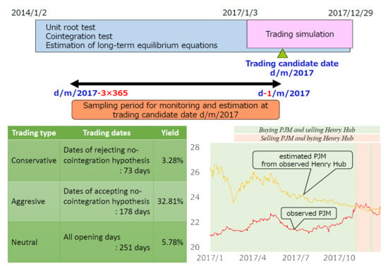
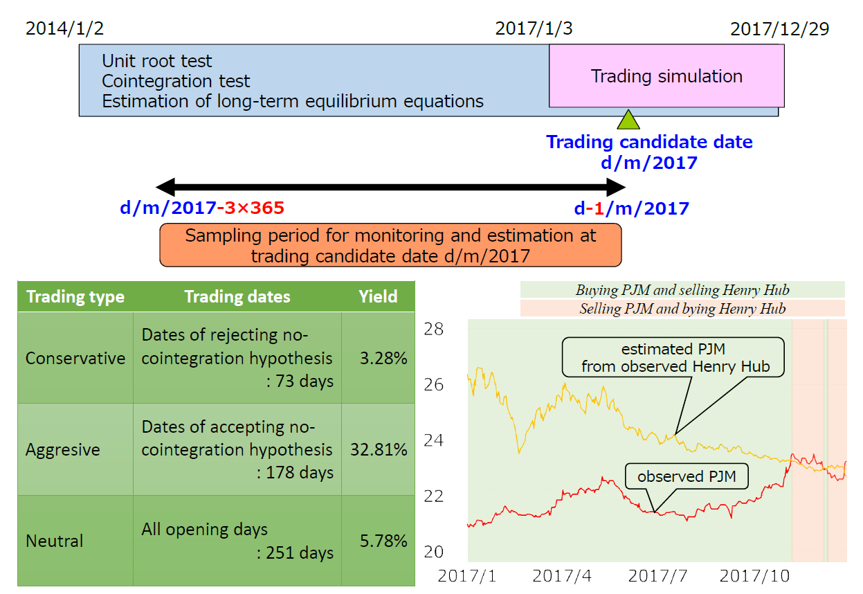
This study employs the PJM Western Hub Real-Time Off-Peak Futures as wholesale power, and the Henry Hub Natural Gas Futures as natural gas from the viewpoint of liquidity and representativeness. Both futures are listed on the NYMEX, which is one of the most efficient commodity exchanges in the world. We use daily data from 2 January 2014 to 29 December 2017, which are obtained from Bloomberg. Shale gas fields developed significantly from 2008 to 2013. At the same time, thermal power generation costs declined. To avoid this structural change, this study uses data from 2014. The long-term equilibrium equation at the trading candidate date is estimated by using three years of observations up to the day before that day. Therefore, the simulation test period is for only one year in 2017.
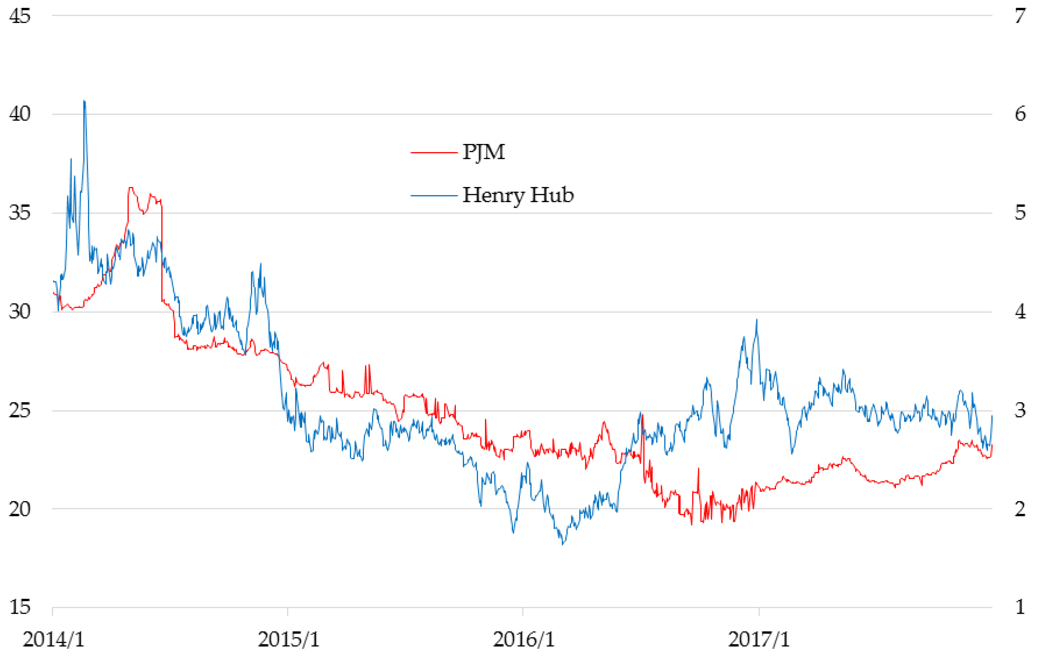
Table 1 presents the summary statistics of Henry Hub and PJM. Each number of observations is 1007, because the NYMEX was open for 1007 days from 2 January 2014 to 29 December 2017. We reject the hypothesis that both variables are normally distributed by the Jarque–Bera statistics calculated from the skewness and kurtosis. Table 2 presents the results obtained from the KPSS test, ADF test, and PP test. The KPSS test rejects the null hypothesis that these variables are stationary, and accepts the null hypothesis that the first differences of these variables are stationary. Both the ADF test and the PP test accept the null hypothesis that these variables have a unit root, and reject the null hypothesis that the first differences of these variables have a unit root. Moreover, Figure 2 provides the time plots of each variable. Intuitively, it seems that the Henry Hub and PJM are interlocked.
4. Results of Analyses and Simulations
4.1. Unit Root Tests
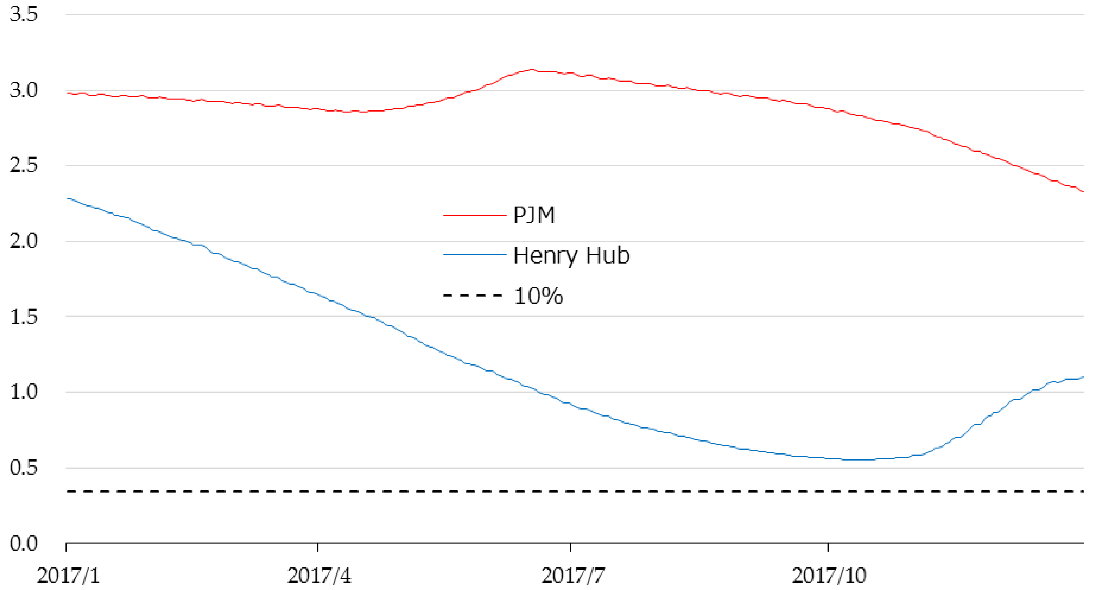
Figure 3 presents the KPSS test statistics for 2017. The test statistic on a certain day t is obtained during the sample period from t − 3 × 365 to t − 1. The stationary hypotheses of both variables are rejected by all the tests during the period. In other words, while each of these two variables is unit root tested 365 times using approximately 750 samples, we can accept the unit root hypothesis by all KPSS tests.
4.2. Cointegration Tests
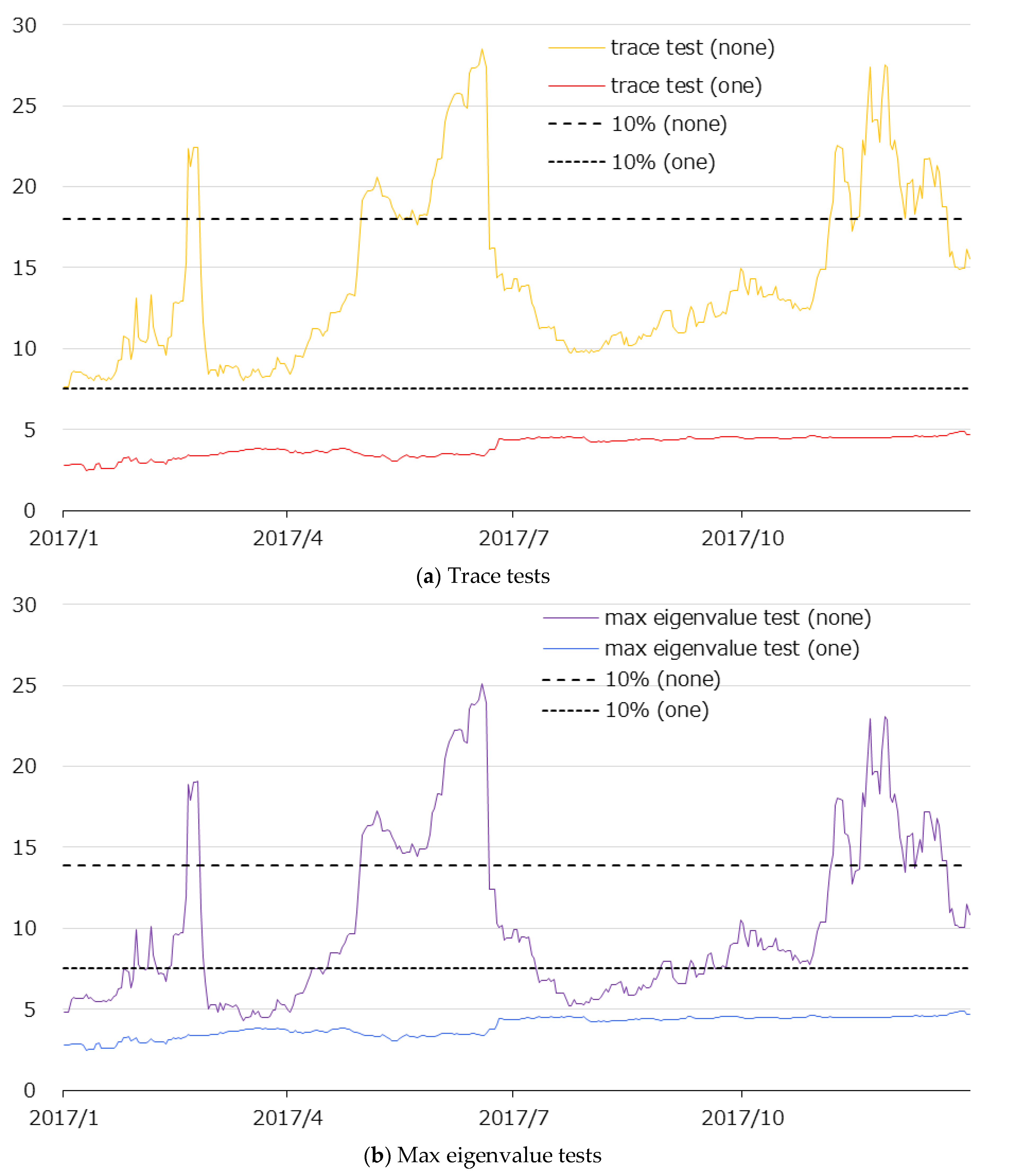
Figure 4a,b present the trace test statistics and maximum eigenvalue test statistics of Johansen (1988) tests in 2017, respectively. As with above unit root tests, each test statistic on a certain day t is obtained during the sample period from t − 3 × 365 to t − 1. Figure 4 shows that both trace test results and maximum eigenvalue test results tend to be similar.
In testing for null hypothesis of cointegration, both the trace test and the max eigenvalue test accept the null over the entire period of 2017. Each test with approximately 750 samples is conducted 365 times, and all results accept the null hypothesis.
In testing for the null hypothesis of no cointegration, the null hypothesis cannot be rejected 103 times out of 365 times. We may consider that the relatively small number of samples, the short-term trend of the prices, and the nonlinearity of the real structure cause these results, although these variables are in fact a cointegrating relationship.
4.3. Selection of Trading Dates
The selection of the trading dates depends on the test results related to the relationship between both variables.
First, we define the period when the null hypothesis of no cointegration is rejected by the Johansen (1988) test as period A, and the period that is accepted as period B. Next, the three strategies for trading only in period A, only in period B, and in both periods are defined as conservative, aggressive, and neutral types, respectively. Finally, we simulate these three trading strategies and examine their impact on profitability.
An explanation of each trading strategy and pre-prediction characteristics are shown in Table 3. We refer to period A as a continued tendency for the deviation from the equilibrium to be small and to converge to an equilibrium state in a short time. Therefore, we predict as follows: the conservative type has a disadvantage in that trading opportunities are limited and yield is low.
We consider that in period B, the large deviation from the equilibrium tends to continue for a long time. Therefore, we forecast that the aggressive type has high yield. The interpretation of the neutral type is a moderation of the conservative type and the aggressive type. The neutral type has an exclusive advantage in that all opening days are trading opportunities, although its return is considered to be average.
There are 251 opening days in 2017 when the current simulation is conducted. As a breakdown, periods A and B comprise 73 days and 178 days, respectively.
4.4. Estimation of Long-Term Equilibrium Equation
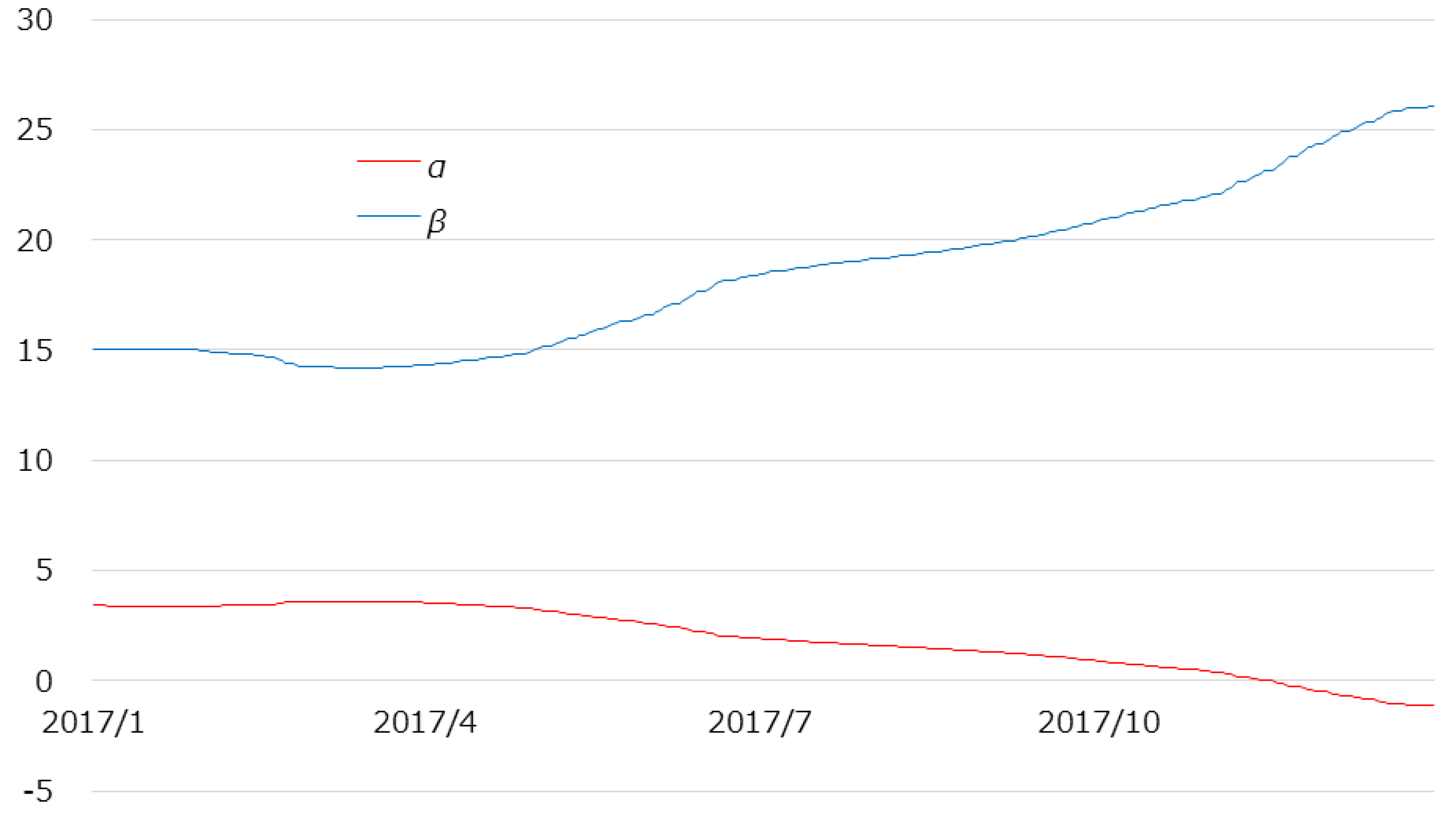
Figure 5 provides the time plots of the coefficients of long-term equilibrium Equation (1). These generally change gradually. In other words, the structure seems to change gradually. This study’s trading strategy is based on slow structural change and short-term inefficiency, and therefore, we can expect to earn profits unless we hold one position for a long time.
After the simulation, we determine appropriate lead and lag orders based on the Schwarz information criterion in order to estimate the coefficients by DOLS. As a result, we select lead order 0 and lag order 1 in approximately 98% of the simulation period. In other words, Equation (2) is the appropriate equilibrium formula.
4.5. Simulations
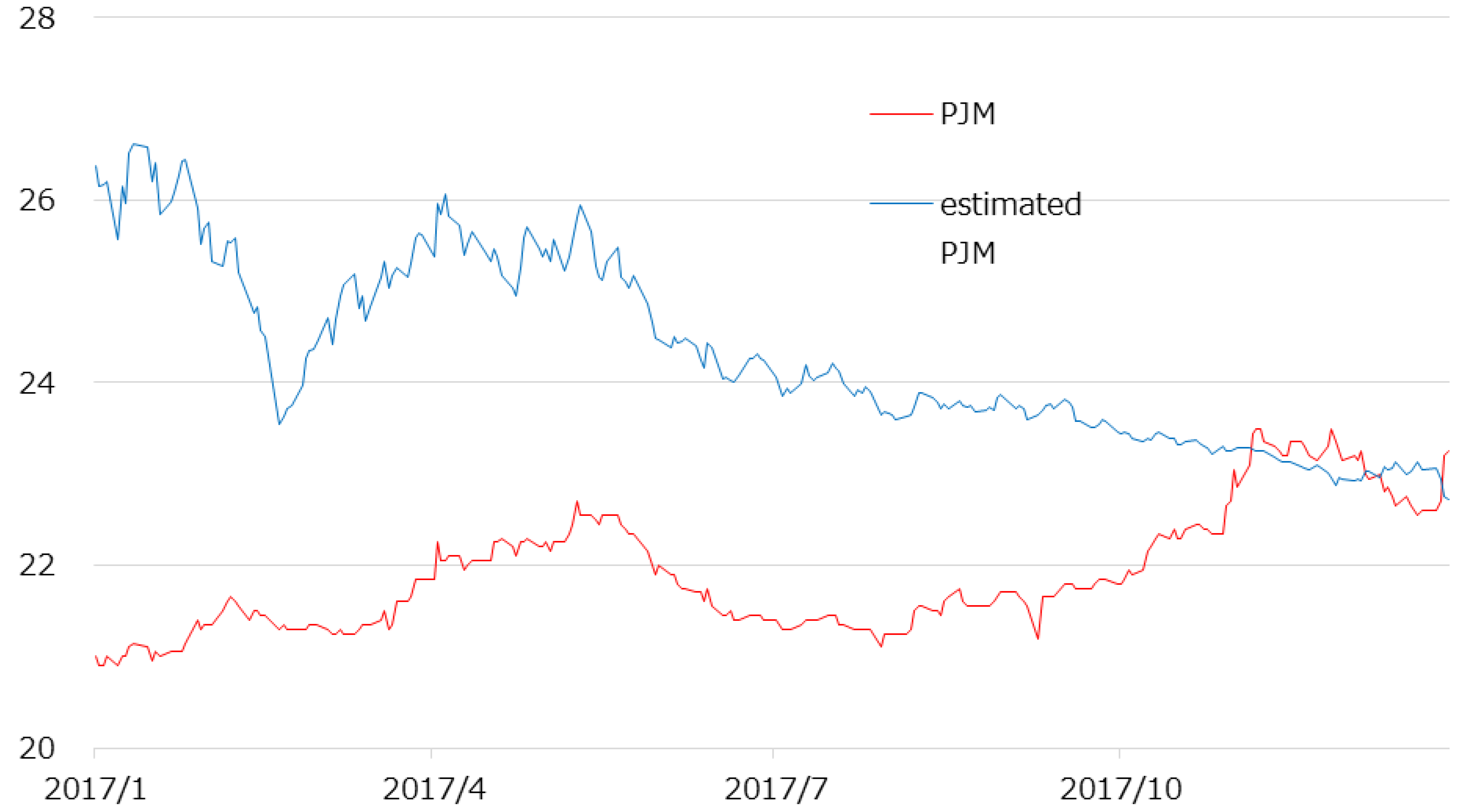
Figure 6 provides the observed PJM value and the PJM value estimated from the observed value of the Henry Hub by using daily equilibrium Equation (1). When the estimated PJM is higher than the observed PJM, we interpret this as the Henry Hub being higher than the PJM. Therefore, we take a long position in the PJM and a short position in the Henry Hub. Conversely, when the estimated PJM is lower than the observed PJM, we may consider that the Henry Hub is lower than the PJM is. Therefore, we take a short position in the PJM and a long position in the Henry Hub. The positions were inverted three times in this simulation. In the case of the neutral type, with the whole period as the trading day, we liquidate our position three times.
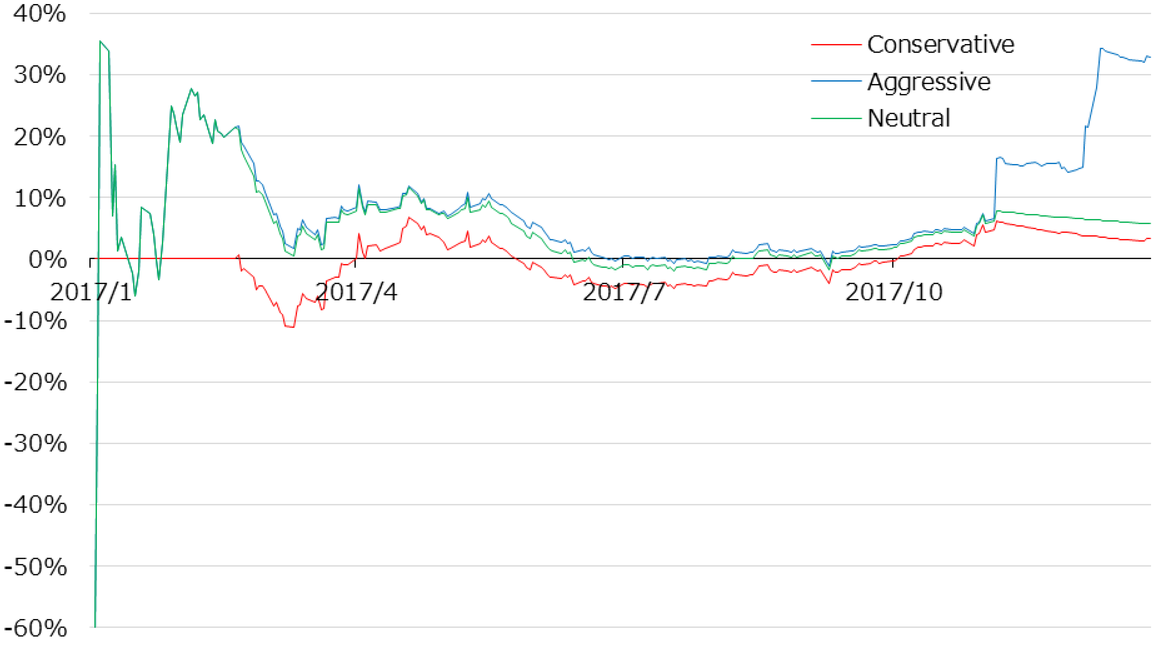
Table 4 presents the results of the simulation. We must take a new position on the selected trading date, and therefore, a cumulative position equals the number of selected trading dates. Before the simulation, we forecast that the yield of the aggressive type is the largest while that of the conservative type is the smallest. Figure 7 provides the time plots of each yield. Each trading strategy has a negative yield for only a very short time. Moreover, all yields have almost the same tendency.
5. Discussion
We present profitability by statistical arbitrage trading using a very primitive algorithm based on a long-term equilibrium formula between wholesale electricity futures and natural gas futures.
This study demonstrates the possibility of earning profit by statistical arbitrage between PJM wholesale electricity futures and Henry Hub natural gas futures by trading simulations based on an algorithm using the equilibrium equation estimated daily. From this, we derive the following two hypotheses. First, statistical arbitrage opportunities continue for a relatively long time, because there are not many arbitrage dealers that utilize the long-term equilibrium between these variables. It can be assumed that most traders of these two kinds of futures are energy companies that hedge profits by considering the cost and profit structure, while institutional investors that conduct pair trade among energy derivatives are extremely limited. The second hypothesis is that there is no sudden structural change in the sample period of this study. This is obvious, because the equilibrium equation estimated by the daily data can capture the market structure change. After all, it can be said that there is profitability through daily statistical arbitrage trading, if we can find cointegrated securities without a steep market structure change, earlier than other traders.
However, the problems with the simulation are fourfold, and should be addressed by further study. First, it is insufficient in terms to confirm the robustness of the trading strategy, because the simulation in this study is based on historical data for only one year. In the context of this study, the robustness does not include academic appropriateness of long-run equilibrium between these economic variables, but means practical profitability of the trading strategy, which allows losses within the range specified by the trader. The robustness should be confirmed by Monte Carlo simulation of this trading methodology in data-generating processors or artificial markets that simulate real price fluctuations.
Second, it is expected that the method adopted in this study cannot respond to rapid market structural change. Although the simulations in this sample period, which has a modest market structural change, can show the profitability, it is uncertain whether the change amounts to a deficit or a surplus if these prices fluctuate rapidly, like in bubbles or crashes. We may need to develop trading strategies based on the estimation of the spread using high frequency data or an algorithm to detect sudden changes in the market structure to stop trading.
Third, although three kinds of algorithms are tested, these algorithms cannot maximize the returns. The trading strategy for the maximization of returns under appropriate risk management should be able to be developed by changing the sample period to estimate the long-term equilibrium and the position depending on deviation from the long-term equilibrium. This study adopts estimation of long-term equilibrium formula over three years and daily trading with fixed size.
Finally, this study does not consider the constraints of actual exchange at all. In other words, this study assumes the unrealistic conditions in which the contract units are not restricted and trading is possible at the prices of the historical data. Each exchange standardizes the contract specifications for each commodity, and therefore, we cannot adjust the contract units depending on the prices. Furthermore, actual transactions need transaction costs. It is impossible to avoid changing prices owing to own orders. Buying causes price increases, and selling causes price drops. Apart from this, real transactions need real cash, including trading fees. Moreover, this study assumes that traders can constantly and permanently increase their positions. In other words, they can take their positions, which need their infinite credit. These are impossible conditions for risk management.
These realistic tasks on commodity futures trading are unavoidable for practitioners, but tend to be avoided academically. We hope that further study of commodity markets will be promoted from various academic viewpoints.
Funding
This research received no external funding.
Acknowledgments
The author would like to thank Editage (www.editage.jp) for English language editing, and the anonymous reviewers, whose valuable comments helped to improve an earlier version of this paper.
Conflicts of Interest
The author declares no conflict of interest.
References
- Alexakis, Christos. 2010. Long-run relations among equity indices under different market conditions: Implications on the implementation of statistical arbitrage strategies. Journal of International Financial Markets, Institutions and Money 20: 389–403. [Google Scholar] [CrossRef]
- Asche, Frank, Petter Osmundsen, and Maria Sandsmark. 2006. The UK market for natural gas, oil and electricity: Are the prices decoupled? The Energy Journal 27: 27–40. [Google Scholar] [CrossRef]
- Baviera, Raviera, and Tommaso Santagostino Baldi. 2018. Stop-loss and leverage in optimal statistical arbitrage with an application to energy market. Energy Economics. forthcoming. [Google Scholar] [CrossRef] [Green Version]
- Emery, Gary W., and Qingfeng Wilson Liu. 2002. An analysis of the relationship between electricity and natural-gas futures prices. The Journal of Futures Markets 22: 95–122. [Google Scholar] [CrossRef]
- Focardi, Sergio M., Frank J. Fabozzi, and Ivan K. Mitov. 2016. A new approach to statistical arbitrage: Strategies based on dynamic factor models of prices and their performance. Journal of Banking & Finance 65: 134–55. [Google Scholar] [CrossRef]
- Freitas, Carlos J. Pereira, and Patrícia Pereira da Silva. 2015. European Union emissions trading scheme impact on the Spanish electricity price during phase II and phase III implementation. Utilities Policy 33: 54–62. [Google Scholar] [CrossRef] [Green Version]
- Furió, Dolores, and Helena Chuliá. 2012. Price and volatility dynamics between electricity and fuel costs: Some evidence for Spain. Energy Economics 34: 2058–65. [Google Scholar] [CrossRef]
- Gautam, Tej K., and Krishna P. Paudel. 2018. Estimating sectoral demands for electricity using the pooled mean group method. Applied Energy 231: 54–67. [Google Scholar] [CrossRef]
- Hain, Martin, Julian Hess, and Marliese Uhrig-Homburg. 2018. Relative value arbitrage in European commodity markets. Energy Economics 69: 140–54. [Google Scholar] [CrossRef]
- Haugom, Erik, Guttorm A. Hoff, Peter Molnár, Maria Mortensen, and Sjur Westgaard. 2014. The forecasting power of medium-term futures contracts. Journal of Energy Markets 7: 1–23. [Google Scholar] [CrossRef]
- Haugom, Erik, Guttorm A. Hoff, Peter Molnár, Maria Mortensen, and Sjur Westgaard. 2018. The forward premium in the Nord Pool Power market. Emerging Markets Finance and Trade 54: 1793–807. [Google Scholar] [CrossRef]
- Joëts, Marc, and Valérie Mignon. 2011. On the link between forward energy prices: A nonlinear panel cointegration approach. Energy Economics 34: 1170–75. [Google Scholar] [CrossRef]
- Johansen, Søren. 1988. Statistical analysis of cointegration vectors. Journal of Economic Dynamics and Control 12: 231–54. [Google Scholar] [CrossRef]
- Kwiatkowski, Denis, Peter C. B. Phillips, Peter Schmidt, and Yongcheol Shin. 1992. Testing the null hypothesis of stationarity against the alternative of a unit root. Journal of Econometrics 54: 159–78. [Google Scholar] [CrossRef]
- Liu, Guo-Dong, and Chi-Wei Su. 2018. The dynamic causality between gold and silver prices in China market: A rolling window bootstrap approach. Finance Research Letters. forthcoming. [Google Scholar] [CrossRef]
- Mayordomo, Sergio, Juan Ignacio Peña, and Juan Romo. 2014. Testing for statistical arbitrage in credit derivatives markets. Journal of Empirical Finance 26: 59–75. [Google Scholar] [CrossRef]
- Mjelde, James W., and David A. Bessler. 2009. Market integration among electricity markets and their major fuel source markets. Energy Economics 31: 482–91. [Google Scholar] [CrossRef]
- Mohammadi, Hassan. 2009. Electricity prices and fuel costs: Long-run relations and short-run dynamics. Energy Economics 31: 503–9. [Google Scholar] [CrossRef]
- Phillips, Peter C., and Pierre Perron. 1988. Testing for a unit root in time series regression. Biometrika 75: 335–46. [Google Scholar] [CrossRef]
- Serletis, Apostolos, and John Herbert. 1999. The message in North American energy prices. Energy Economics 21: 471–83. [Google Scholar] [CrossRef]
- Serletis, Apostolos, and Akbar Shahmoradi. 2006. Measuring and testing natural gas and electricity markets volatility: Evidence from Alberta’s deregulated markets. Studies in Nonlinear Dynamics & Econometrics 10: 1341. [Google Scholar] [CrossRef]
Figure 1.
Open interests of WTI futures and Henry Hub futures.

Figure 2.
Prices of PJM futures and Henry Hub futures.

Figure 3.
KPSS tests.

Figure 4.
Johansen tests.

Figure 5.
Coefficients of equilibrium equation.

Figure 6.
Observed PJM and estimated PJM from observed Henry Hub.

Figure 7.
Yield.


Table 1.
Summary statistics.
| Statistic | Henry Hub | PJM |
|---|---|---|
| Observations | 1007 | 1007 |
| Mean | 3.115 | 24.81 |
| Median | 2.925 | 23.35 |
| Maximum | 6.149 | 36.30 |
| Minimum | 1.639 | 19.20 |
| Standard deviation | 0.794 | 3.879 |
| Skewness | 0.777 | 1.050 |
| Kurtosis | 3.283 | 3.542 |
| Jarque–Bera | 104.8 [0.00] | 197.4 [0.00] |
Note: Values in brackets indicate p-values.
Table 2.
Unit root tests.
| Test | Henry Hub | First Differences of Henry Hub | PJM | First Differences of PJM |
|---|---|---|---|---|
| KPSS | 1.724 (0.463) * | 0.116 (0.463) | 3.176 (0.463) * | 0.149 (0.463) |
| ADF | −2.235 (−2.864) | −32.719 (−2.864) ** | −1.627 (−2.864) | −41.267 (−2.864) ** |
| PP | −2.015 (−2.864) | −33.348 (−2.864) ** | −1.645 (−2.864) | −41.743 (−2.864) ** |
Note: Values in parentheses are 5% critical values. * indicates that the stationary hypothesis is rejected at the 5% significance level. ** indicates that the unit root hypothesis is rejected at the 5% significance level.
Table 3.
Trading types.
| Characteristics | Conservative | Aggressive | Neutral |
|---|---|---|---|
| Trading dates | Dates of rejecting no-cointegration hypothesis | Dates of accepting no-cointegration hypothesis | All opening days |
| Concept of trading date selection | Only when convergence to equilibrium is expected in a short time | Only when deviation from equilibrium continues | Whenever deviation from equilibrium occurs |
| Opportunities | Occasionally | Frequently | Always |
| Yield | Low | High | Medium |
Table 4.
Simulation results.
| Characteristics | Conservative | Aggressive | Neutral |
|---|---|---|---|
| Cumulative position | 73 | 178 | 251 |
| Profit | 2.363 | 57.271 | 14.263 |
| Yield | 3.28% | 32.81% | 5.78% |
© 2019 by the author. Licensee MDPI, Basel, Switzerland. This article is an open access article distributed under the terms and conditions of the Creative Commons Attribution (CC BY) license (http://creativecommons.org/licenses/by/4.0/).
Share and Cite
MDPI and ACS Style
Nakajima, T. Expectations for Statistical Arbitrage in Energy Futures Markets. J. Risk Financial Manag. 2019, 12, 14. https://doi.org/10.3390/jrfm12010014
AMA Style
Nakajima T. Expectations for Statistical Arbitrage in Energy Futures Markets. Journal of Risk and Financial Management. 2019; 12(1):14. https://doi.org/10.3390/jrfm12010014
Chicago/Turabian StyleNakajima, Tadahiro. 2019. "Expectations for Statistical Arbitrage in Energy Futures Markets" Journal of Risk and Financial Management 12, no. 1: 14. https://doi.org/10.3390/jrfm12010014