Estimating Mixture Entropy with Pairwise Distances

1
Santa Fe Institute, Santa Fe, NM 87501, USA
2
Department of Aeronautics and Astronautics, Massachusetts Institute of Technology, Cambridge, MA 02139, USA
*
Author to whom correspondence should be addressed.
Entropy 2017, 19(7), 361; https://doi.org/10.3390/e19070361
Submission received: 8 June 2017
/
Revised: 8 July 2017
/
Accepted: 12 July 2017
/
Published: 14 July 2017
(This article belongs to the Special Issue Information Theory in Machine Learning and Data Science)
Abstract
:Mixture distributions arise in many parametric and non-parametric settings—for example, in Gaussian mixture models and in non-parametric estimation. It is often necessary to compute the entropy of a mixture, but, in most cases, this quantity has no closed-form expression, making some form of approximation necessary. We propose a family of estimators based on a pairwise distance function between mixture components, and show that this estimator class has many attractive properties. For many distributions of interest, the proposed estimators are efficient to compute, differentiable in the mixture parameters, and become exact when the mixture components are clustered. We prove this family includes lower and upper bounds on the mixture entropy. The Chernoff -divergence gives a lower bound when chosen as the distance function, with the Bhattacharyaa distance providing the tightest lower bound for components that are symmetric and members of a location family. The Kullback–Leibler divergence gives an upper bound when used as the distance function. We provide closed-form expressions of these bounds for mixtures of Gaussians, and discuss their applications to the estimation of mutual information. We then demonstrate that our bounds are significantly tighter than well-known existing bounds using numeric simulations. This estimator class is very useful in optimization problems involving maximization/minimization of entropy and mutual information, such as MaxEnt and rate distortion problems.
1. Introduction
A mixture distribution is a probability distribution whose density function is a weighted sum of individual densities. Mixture distributions are a common choice for modeling probability distributions, in both parametric settings, for example, learning a mixture of Gaussians statistical model [1], and non-parametric settings, such as kernel density estimation.
It is often necessary to compute the differential entropy [2] of a random variable with a mixture distribution, which is a measure of the inherent uncertainty in the outcome of the random variable. Entropy estimation arises in image retrieval tasks [3], image alignment and error correction [4], speech recognition [5,6], analysis of debris spread in rocket launch failures [7], and many other settings. Entropy also arises in optimization contexts [4,8,9,10], where it is minimized or maximized under some constraints (e.g., MaxEnt problems). Finally, entropy also plays a central role in minimization or maximization of mutual information, such as in problems related to rate distortion [11].
Unfortunately, in most cases, the entropy of a mixture distribution has no known closed-form expression [12]. This is true even when the entropy of each component distribution does have a known closed-form expression. For instance, the entropy of a Gaussian has a well-known form, while the entropy of a mixture of Gaussians does not [13]. As a result, the problem of finding a tractable and accurate estimate for mixture entropy has been described as “a problem of considerable current interest and practical significance” [14].
One way to approximate mixture entropy is with Monte Carlo (MC) sampling. MC sampling provides an unbiased estimate of the entropy, and this estimate can become arbitrarily accurate by increasing the number of MC samples. Unfortunately, MC sampling is very computationally intensive, as, for each sample, the (log) probability of the sample location must be computed under every component in the mixture. MC sampling typically requires a large number of samples to estimate entropy, especially in high-dimensions. Sampling is thus typically impractical, especially for optimization problems where, for every parameter change, a new entropy estimate is required. Alternatively, it is possible to approximate entropy using numerical integration, but this is also computationally expensive and limited to low-dimensional applications [15,16].
Instead of Monte Carlo sampling or numerical integration, one may use an analytic estimator of mixture entropy. Analytic estimators have estimation bias but are much more computationally efficient. There are several existing analytic estimators of entropy, discussed in-depth below. To summarize, however, commonly-used estimators have significant drawbacks: they have large bias relative to the true entropy, and/or they are invariant to the amount of “overlap” between mixture components. For example, many estimators do not depend on the locations of the means in a Gaussian mixture model.
In this paper, we introduce a novel family of estimators for the mixture entropy. Each member of this family is defined via a pairwise-distance function between component densities. The estimators in this family have several attractive properties. They are computationally efficient, as long as the pairwise-distance function and the entropy of each component distribution are easy to compute. The estimation bias of any member of this family is bounded by a constant. The estimator is continuous and smooth and is therefore useful for optimization problems. In addition, we show that when the Chernoff -divergence (i.e., a scaled Rényi divergence) is used as a pairwise-distance function, the corresponding estimator is a lower-bound on the mixture entropy. Furthermore, among all the Chernoff -divergences, the Bhattacharrya distance () provides the tightest lower bound when the mixture components are symmetric and belong to a location family (such as a mixture of Gaussians with equal covariances). We also show that when the Kullback–Leibler [KL] divergence is used as a pairwise-distance function, the corresponding estimator is an upper-bound on the mixture entropy. Finally, our family of estimators can compute the exact mixture entropy when the component distributions are grouped into well-separated clusters, a property not shared by other analytic estimators of entropy. In particular, the bounds mentioned above converge to the same value for well-separated clusters.
The paper is laid out as follows. We first review mixture distributions and entropy estimation in Section 2. We then present the class of pairwise distance estimators in Section 3, prove bounds on the error of any estimator in this class, and show distance functions that bound the entropy as discussed above. In Section 4, we consider the special case of mixtures of Gaussians, and give explicit expressions for lower and upper bounds on the mixture entropy. When all the Gaussian components have the same covariance matrix, we show that these bounds have particularly simple expressions. In Section 5, we consider the closely related problem of estimating the mutual information between two random variables, and show that our estimators can be directly used to estimate and bound the mutual information. For the Gaussian case, these can be used to bound the mutual information across a type of Additive White Noise Gaussian channel. Finally, in Section 6, we run numerical experiments and compare the performance of our lower and upper bounds relative to existing estimators. We consider both mixtures of Gaussians and mixtures of uniform distributions.
2. Background and Definitions
We consider the differential entropy of a continuous random variable X, defined as
where is a mixture distribution,
and where indicates the weight of component i (, ) and the probability density of component i.
We can treat the set of component weights as the probabilities of outcomes of a discrete random variable C, where . Consider the mixed joint distribution of the discrete random variable C and the continuous random variable X,
and note the following identities for conditional and joint entropy [17],
where we use H for discrete and differential entropy interchangeably. Here, the conditional entropies are defined as
Using elementary results from information theory [2], can be bounded from below by
since conditioning can only decrease entropy. Similarly, can be bounded from above by
following from and the non-negativity of the conditional discrete entropy . This upper bound on the mixture entropy was previously proposed by Huber et al. [18].
It is easy to see that the bound in Equation (1) is tight when all the components have the same distribution, since then for all i. The bound in Equation (2) becomes tight when , i.e., when any sample from uniquely determines the component identity C. This occurs when the different mixture components have non-overlapping supports, for all x and . More generally, the bound of Equation (2) becomes increasingly tight as the mixture distributions move farther apart from one another.
In the case where the entropy of each component density, for , has a simple closed form expression, the bounds in Equations (1) and (2) can be easily computed. However, neither bound depends on the “overlap” between components. For instance, in a Gaussian mixture model, these bounds are invariant to changes in the component means. The bounds are thus unsuitable for many problems; for instance, in optimization, one typically tunes parameters to adjust component means, but the above entropy bounds remain the same regardless of mean location.
There are two other estimators of the mixture entropy that should be mentioned. The first estimator is based on kernel density estimation [16,19]. It estimates the entropy using the mixture probability of the component means, ,
The second estimator is a lower bound that is derived using Jensen’s inequality [2], , giving
In the literature, the term has been referred to as the “Cross Information Potential” [20,21] and the “Expected Likelihood Kernel” [22,23] (ELK, we use this second acronym to label this estimator). When the component distributions are Gaussian, , the ELK has a simple closed-form expression,
where each is a Gaussian defined as . This lower bound was previously proposed for Gaussian mixtures in [18] and in a more general context in [12].
Both , Equation (3), and , Equation (5), are computationally efficient, continuous and differentiable, and depend on component overlap, making them suitable for optimization. However, as will be shown via numerical experiments (Section 6), they exhibit significant underestimation bias. At the same time, we will show that for Gaussian mixtures with equal covariance, is only an additive constant away from an estimator in our proposed class.
3. Estimators Based on Pairwise-Distances
3.1. Overview
Let be some (generalized) distance function between probability densities and . Formally, we assume that D is a premetric, meaning that it is non-negative and if . We do not assume that D is symmetric, nor that it obeys the triangle inequality, nor that it is strictly greater than 0 when .
For any allowable distance function D, we propose the following entropy estimator:
This estimator can be efficiently computed if the entropy of each component and for all have simple closed-form expressions. There are many distribution-distance function pairs that satisfy these conditions (e.g., Kullback–Leibler divergence, Renyi divergences, Bregman divergences, f-divergences, etc., for Gaussian, uniform, exponential, etc.) [24,25,26,27,28].
To do so, consider the “smallest” and “largest” allowable distance functions,
For any D and , , thus
3.2. Lower Bound
Note that , where is Rényi divergence of order α [30].
We show that for any , is a lower bound on the entropy (for , is not a valid distance function (see Appendix A)). To do so, we make use of a derivation from [31] and write,
The inequalities (a) and (b) follow from Jensen’s inequality. This inequality is used directly in , while in it follows from
Note that Jensen’s inequality is used in the derivations of both this lower bound as well as the lower bound in Equation (4). However, the inequality is applied differently in the two cases, and, as will be demonstrated in Section 6, the estimators have different performance.
We have shown that using as a distance function gives a lower bound on the mixture entropy for any . For a general mixture distribution, one could optimize over the value of to find the tightest lower bound. However, we can show that the tightest bound is achieved for in the special case when all of the mixture components are symmetric and come from a location family,
Examples of this situation include mixtures of Gaussians with the same covariance (“homoscedastic” mixtures), multivariate t-distributions with the same covariance, location-shifted bounded uniform distributions, most kernels used in kernel density estimation, etc. It does not apply to skewed distributions, such as as the skew-normal distribution [12].
To show that is optimal, first define the Chernoff -coefficient as
We show that for any pair of symmetric distributions from a location family, is minimized by . This means that all pairwise distances are maximized by , and, therefore, the entropy estimator (Equation (6)) is maximized by .
First, define a change of variables
which gives and . This allows us to write the Chernoff -coefficient as
where, in , we have substituted variables, and in we used the assumption that . Since we have shown that , is symmetric in about . In Appendix A, we show that is everywhere convex in . Together, this means that must achieve a minimum value at .
The Chernoff -coefficient for is known as the Bhattacharyya coefficient, with the corresponding Bhattacharyya distance [32] defined as
Since any Chernoff -divergence is a lower bound for the entropy, we write the particular case of Bhattacharyya-distance lower bound as
3.3. Upper Bound
The Kullback–Leibler [KL] divergence [2] is defined as
Using KL divergence as the pairwise distance provides an upper bound on the mixture entropy. We show this as follows:
where indicates expectation when X is distributed according to , indicates the cross-entropy function, and we employ the identity . The inequality in step uses a variational lower bound on the expectation of a log-sum [5,33],
Combining yields the upper bound
3.4. Exact Estimation in the “Clustered” Case
In the previous sections, we derived lower and upper bounds on the mixture entropy, using estimators based on Chernoff -divergence and KL divergence, respectively.
There are situations in which the lower and upper bounds become similar. Consider a pair of component distributions, and . By applying Jensen’s inequality to Equation (9), we can derive the inequality . There are two cases in which a pair of components contributes similarly to the lower and upper bounds. The first case is when is very large, meaning that the KL is also very large. By Equation (6), distances enter into our estimators as , and, in this case, . In the second case, , meaning that must also be near zero, and, in this case, . Thus, the lower and upper bounds become similar when all pairs of components are either very close together or very far apart.
In this section, we analyze this special case. Specifically, we consider the situation when mixture components are “clustered”, meaning that there is a grouping of component distributions such that distributions in the same group are approximately the same and distributions assigned to different groups are very different from one another. We show that in this case our lower and upper bounds become equal and our pairwise-distance estimate of the entropy is tight. Though this situation may seem like an edge case, clustered distributions do arise in mixture estimation, e.g., when there are repeated data points, or as solutions to information-theoretic optimization problems [11]. Note that the number of groups is arbitrary, and therefore this situation includes the extreme cases of a single group (all component distributions are nearly the same) as well as N different groups (all component distributions are very different).
Formally, let the function indicate the group of component i. We define that the components are “clustered” with respect to grouping g iff whenever for some small , and whenever some large . We use the notation to indicate the sum of the weights of the components in group k, where indicates the Kronecker delta function. For technical reasons, below we only consider where is strictly greater than 0.
We show that when is small and is large, both for and approach
Since one is a lower bound and one is an upper bound on the true entropy, the estimators become exact as they converge in value.
Recall that . For , is a monotonically decreasing function for [34], meaning that for . In addition, is a monotonically increasing function for [34], thus for . Using the assumption that and combining gives the bound
for , leading to
In the second line, for the summation over in the same group, we’ve used the non-negativity of .
For the upper bound , we use that for i and j in the same group, and otherwise . This gives the bound
The difference between the bounds is bounded by
where is the number of groups. Thus, the difference decreases at least linearly in and exponentially in . This shows that, in the clustered case, when and is very large, our lower and upper bounds become exact.
It also shows that any distance measure bounded between BD and KL also gives an exact estimate of entropy in the clustered case. Furthermore, the idea behind this proof can be extended to estimators induced by other bounding distances, beyond BD and KL, so as to show that a particular estimator converges to an exact entropy estimate in the clustered case. Note, however, that, for some distribution-distance pairs, the components will never be considered as “clustered”; e.g., the -Chernoff distance for between any two Gaussians is 0, and so a Gaussian mixture distribution will never be considered clustered according to this distance.
Finally, in the perfectly clustered case, we can show that our lower bound, , is at least as good as the Expected Likelihood Kernel lower bound, , as defined in Equation (4). See Appendix B for details.
4. Gaussian Mixtures
Gaussians are very frequently used as components in mixture distributions. Our family of estimators is well-suited to estimating the entropies of Gaussian mixtures, since the entropy of a d-dimensional Gaussian has a simple closed-form expression,
and because there are many distance functions between Gaussians with closed-form expressions (KL divergence, the Chernoff -divergences [35], 2-Wasserstein distance [36,37], etc.). In this section, we consider Gaussian mixtures and state explicit expression for the lower and upper bounds on the mixture entropy derived in the previous section. We also consider these bounds in the special case where all Gaussian components have the same covariance matrix (homoscedastic mixtures).
We first consider the lower bound, , based on the Chernoff -divergence distance function. For two multivariate Gaussians and , this distance is defined as [35]:
(As a warning, note that most sources show erroneous expressions for the Chernoff and/or Rényi -divergence between two multivariate Gaussians, including [27,29,38,39,40], and even a late draft of this manuscript.)
For the upper bound , the KL divergence between two multivariate Gaussians and is
The appropriate lower and upper bounds are found by plugging in Equations (14) and (15) into Equation (6).
These bounds have simple forms when all of the mixture components have equal covariance matrices; i.e., for all i. First, define a transformation in which each Gaussian component is mapped to a different Gaussian , which has the same mean but where the covariance matrix is rescaled by ,
Then, the lower bound of Equation (10) can be written as
This is derived by combining the expressions for , Equation (14), the entropy of a Gaussian, Equation (13), and the Gaussian density function. For a homoscedastic mixture, the tightest lower bound among the Chernoff -divergences is given by , corresponding to the Bhattacharyya distance,
(This is derived above in Section 3.2.)
For the upper bound, when all Gaussians have the same covariance matrix, we again combine the expressions for KL, Equation (15), the entropy of a Gaussian, Equation (13), and the Gaussian density function to give
Note that this is exactly the expression for the kernel density estimator (Equation (3)), plus a dimensional correction. Thus, surprisingly is a reasonable entropy estimator for homoscedastic Gaussian mixtures, since it is only an additive constant away from KL-distance based estimator (which has various beneficial properties, as described above). This may explain why has been used effectively in optimization contexts [4,8,9,10], where the additive constant is often irrelevant, despite lacking a principled justification in terms of being a a bound on entropy.
5. Estimating Mutual Information
It is often of interest, for example in rate distortion and related problems [11], to calculate the mutual information across a communication channel,
where U is the distribution of signals sent across the channel, and X is the distribution of messages received on the other end of the channel. As with mixture distributions, it is often easy to compute , the entropy of the received signal given the sent signal (i.e., the distribution of noise on the channel). The marginal entropy of the received signals, , on the other hand, is often difficult to compute.
In some cases, the distribution of U may be well approximated by a mixture model. In this case, we can estimate the entropy of the received signals, , using our pairwise distance estimators, as discussed in Section 3. In particular, we have the lower bound
and the upper bound,
where is the density of component i, and noting that the terms cancel in the expression.
This also illuminates that the actual pairwise portion of the estimator, is a measure of the mutual information between the random variable specifying the component identity and the random variable distributed as the mixture of the component densities. If the components are identical, this mutual information is zero, since knowing the component identity tells one nothing about the outcome of X. On the other hand, when all of the components are very different from one another, knowing the component that generated X is very informative, giving the maximum amount of information, .
As a practical example, consider a scenario in which U is a random variable representing the outside temperature on any particular day. This temperature is measured with a thermometer with Gaussian measurement noise (the “Additive White Noise Gaussian channel”). This gives our measurement distribution
If the actual temperature U is (approximately or exactly) distributed as a mixture of M Gaussians, each one having mixture weight , mean , and covariance matrix , then X will also be distributed as a mixture of M Gaussians, each with weight , mean , and covariance matrix . We can then use our estimators to estimate the mutual information between the actual temperature, U, and thermometer measurements, X.
6. Numerical Results
In this section, we run numerical experiments and compare estimators of mixture entropy under a variety of conditions. We consider two different types of mixtures, mixtures of Gaussians and mixtures of uniform distributions, for a variety of parameter values. We evaluate the following estimators:
- The true entropy, , as estimated by a Monte Carlo sampling of the mixture model. Two thousand samples were used for each MC estimate for the mixtures of Gaussians, and 5000 samples were used for the mixtures of uniform distributions.
- Our proposed upper-bound, based on the KL divergence, (Equation (12))
- Our proposed lower-bound, based on the Bhattacharyya distance, (Equation (11))
- The kernel density estimate based on the component means, (Equation (3))
- The lower bound based on the “Expected Likelihood Kernel”, (Equation (4))
- The lower bound based on the conditional entropy, (Equation (1))
- The upper bound based on the joint entropy, (Equation (2)).
We show the values of the estimators 1–5 as line plots, while the region between the conditional (6) and joint entropy (7) is shown in shaded green. The code for these figures can be found at [41], and uses the Gonum numeric library [42].
6.1. Mixture of Gaussians
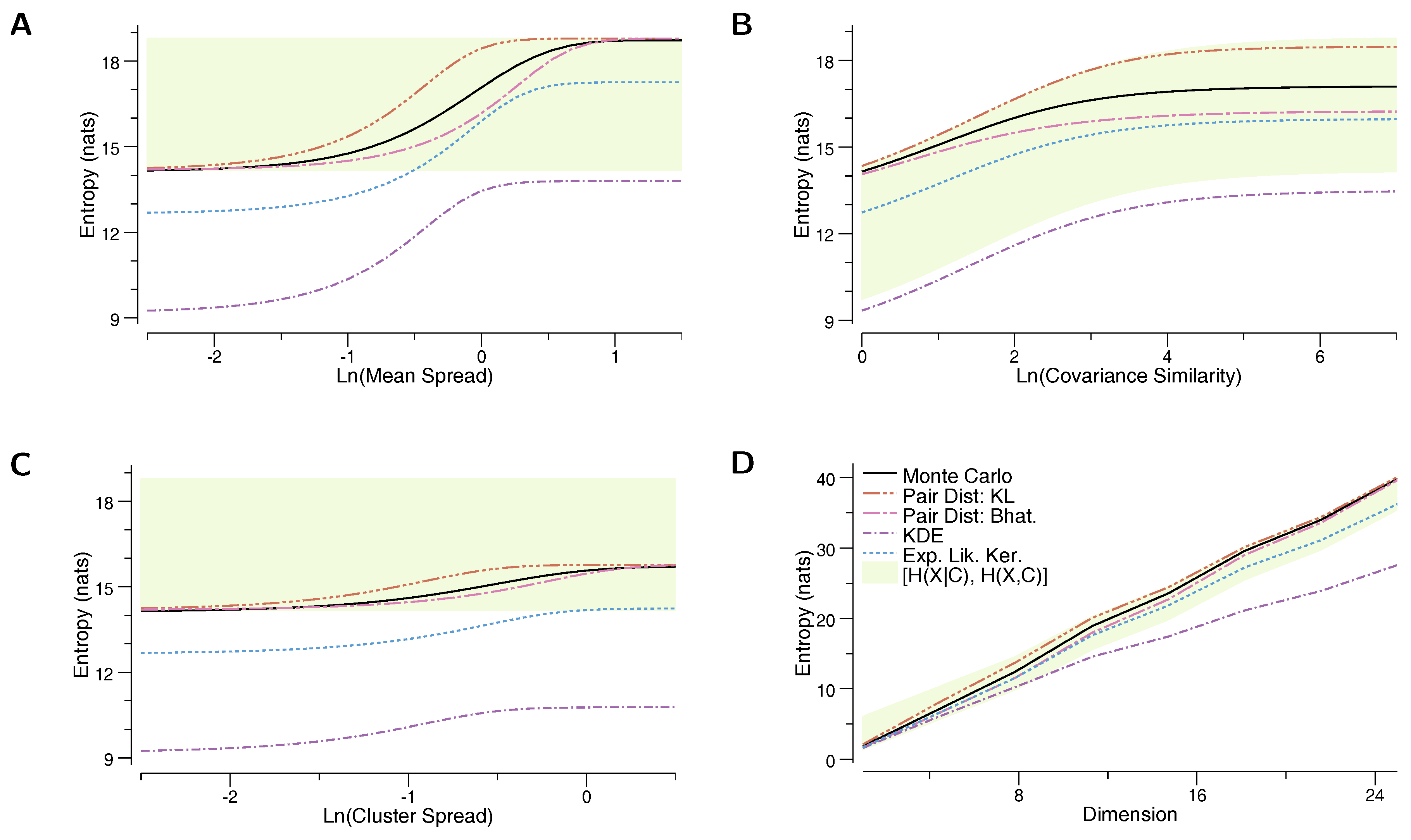
In the first experiment, we evaluate the estimators on a mixture of randomly placed Gaussians, and look at their behavior as the distance between the means of the Gaussians increases. The mixture is composed of 100 10-dimensional Gaussians, each Gaussian distributed as , where indicates the identity matrix. Means are sampled from . Figure 1A depicts the change in estimated entropy as the means grow farther apart, in particular a function of . We see that our proposed bounds are closer to the true entropy than the other estimators over the whole range of values, and in the extremes, our bounds approach the exact value of the true entropy. This is as expected, since as all of the Gaussian mixture components become identical, and as all of the Gaussian components grow very far apart, approaching the case where each Gaussian is in its own “cluster”. The ELK lower bound is a strictly worse estimate than , in this experiment. As expected, the KDE estimator differs by exactly from the KL estimator.
In the second experiment, we evaluate the entropy estimators as the covariance matrices change from less to more similar. We again generate 100 10-dimensional Gaussians. Each Gaussian is distributed as , where now and , where is a Wishart distribution with scale-matrix and n degrees of freedom. Figure 1B compares the the estimators with the true entropy as a function of . When n is small, the Wishart distribution is broad and the covariance matrices differ significantly from one another, while as , all the covariance matrices become close to the identity . Thus, for small n, we essentially recover a “clustered” case, in which every component is in its own cluster and our lower and upper bounds give highly accurate estimates. For large n, we converge to the case of the first experiment.
In the third experiment, we again generate a mixture of 100 10-dimensional Gaussians. Now, however, the Gaussians are grouped into five “clusters”, with each Gaussian component randomly assigned to one of the clusters. We use to indicate the group of each Gaussian’s component , and each of the 100 Gaussians is distributed as . The cluster centers for are drawn from . The results are depicted in Figure 1C as a function of . In the first experiment, we saw that the joint entropy became an increasingly better estimator as the Gaussians grew increasingly far apart. Here, however, we see that there is a significant difference between and the true entropy, even as the groups become increasingly separated. Our proposed bounds, on the other hand, provide accurate estimates of the entropy across the entire parameter sweep. As expected, they become exact in the limit when all clusters are at the same location, as well as when all clusters are very far apart from each other.
Finally, we evaluate the entropy estimators while changing the dimension of the Gaussian components. We again generate 100 Gaussian components, each distributed as , with . We vary the dimensionality d from 1 to 60. The results are shown in Figure 1D. First, we see that when , the KDE estimator and the KL-divergence based estimator give a very similar prediction (differing only by ), but as the dimension increases, the two estimates diverge at a rate of . Similarly, grows increasingly less accurate as the dimension increases. Our proposed lower and upper bounds provide good estimates of the mixture entropy across the whole sweep across dimensions.
As previously mentioned, our lower and upper bounds tend to perform best at the “extremes” and worse in the intermediate regimes. In particular, in Figure 1A,C,D, the distances between component means increase from left to right. On the left hand side of these figures, all of the component means are close and the component distributions overlap, as evidenced by the fact that the mixture entropy is , i.e., . In this regime, when there is essentially a single “cluster”, and our bounds become tight (see Section 3.4). On the right hand side of these figures, the components’ means are all far apart from each other, and the mixture entropy , i.e., (in Figure 1C, it is the five clusters that become far apart, and the mixture entropy ). In this regime where there are many well-separated clusters, our bounds again become tight. In between these two extremes, however, there is no clear clustering of the mixture components, and the entropy bounds are not as tight.
As noted in the previous paragraph, the extremes in three out of the four subfigures approach the perfectly clustered case. In this situation, we show in Appendix B that the BD-based estimator is a better bound on the true entropy than the Expected Likelihood Kernel estimator. We see confirmation of this in the experimental results, where performs worse than the pairwise-distance based estimators.
6.2. Mixture of Uniforms
In the second set of experiments, we consider a mixture of uniform distributions. Unlike Gaussians, uniform distributions are bounded within a hyper-rectangle and do not have full support over the domain. In particular, a uniform distribution over d dimensions is defined as
where x, a, and b are d-dimensional vectors, and the subscript refers to value of x on dimension i. Note that when is a mixture of uniforms, there can be significant regions where , but for some i.
Here, we list the formulae for pairwise distance measure between uniform distributions. In the following, we use to indicate the “volume” of distribution . Uniform components have a constant over their support, and so for all x where . Similarly, we use as the “volume of overlap” between and , i.e., the volume of the intersection of the support of and , . The distance measures between uniforms are then
Like the Gaussian case, we run four different computational experiments and compare the mixture entropy estimates to the true entropy, as determined by Monte Carlo sampling.
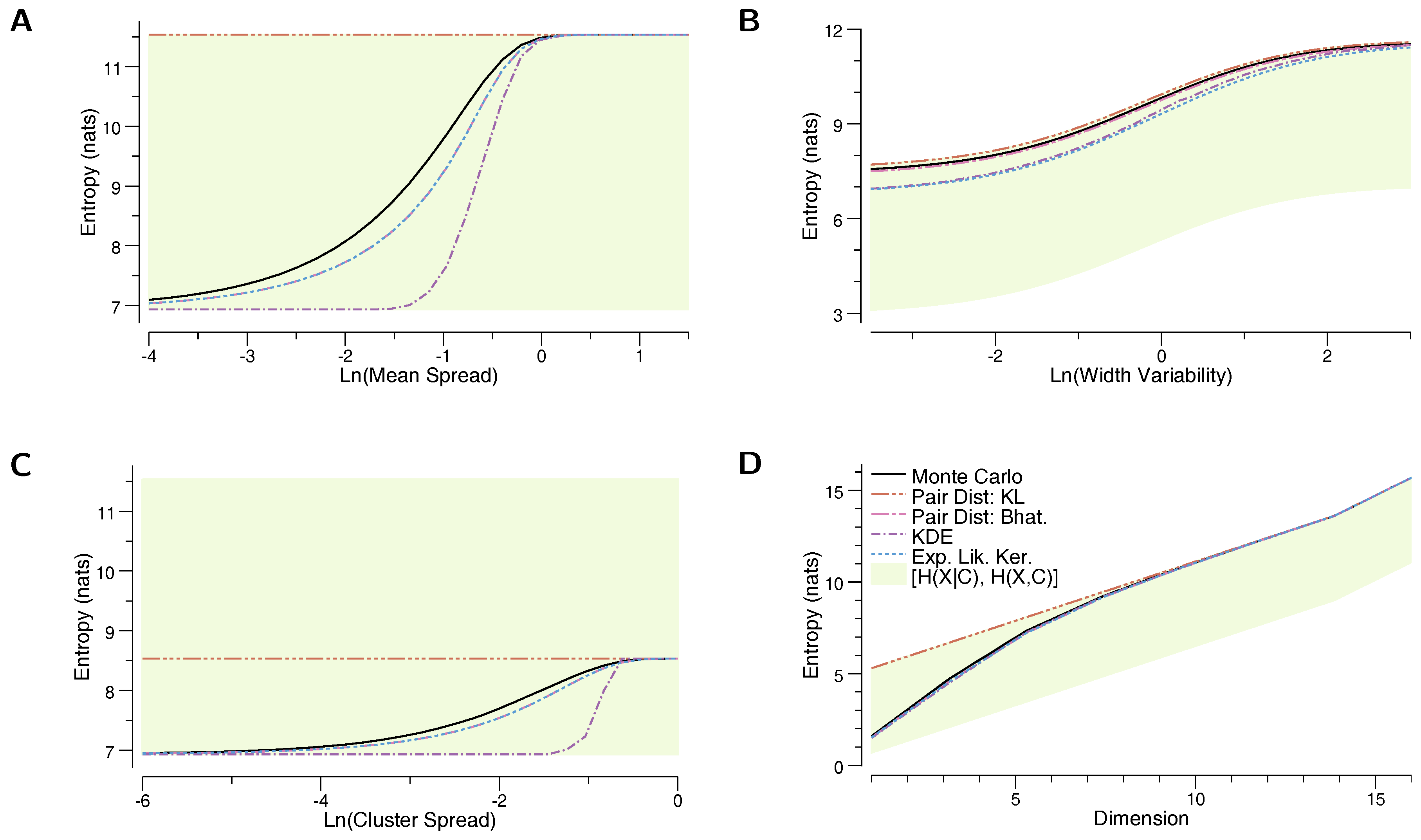
In the first experiment, the mixture consists of 100 10-dimensional uniform components, with , and , where refers to a d-dimensional vector of 1s. Figure 2A depicts the change in entropy as a function of . For very small , the distributions are almost entirely overlapping, while for large they tend very far apart. As expected, the entropy increases with . Here, we see that the prediction of is identical to , which arises because is infinite whenever the support of is not entirely contained in the support of . Uniform components with equal size and non-equal means must have some region of non-overlap, and so the KL is infinite between all pairs of components, thus KL is effectively (Equation (8)). In contrast, we see that estimates the true entropy quite well. This example demonstrates that getting an accurate estimate of mixture entropy may require selecting a distance function that works will with the component distributions. Finally, it turns out that, for uniform components of equal size, . This can be seen by combining Equations (6) and (16), and comparing to Equation (17) (note that when the components have equal size).
In the second experiment, we adjust the variance in the size of the uniform components. We again use 100 10-dimensional components, , where , and , where is the Gamma distribution with shape parameter and rate parameter . Figure 2B shows the change in entropy estimates as a function of . When is small, the sizes have significant spread, while as grows the distributions become close to equally sized. We again see that is a good estimator of entropy, outperforming all of the other estimators. Generally, not all supports will be non-overlapping, so will not necessarily be equal to , though we find the two to be numerically quite close. In this experiment, we find that the lower and upper bounds specified by and provide a tight estimate of the true entropy.
In the third experiment, we again consider a clustered mixture, and evaluate the entropy estimators as these clusters grow apart. Here, there are 100 components with , where is the randomly assigned cluster identity of component i. The cluster centers for are generated according to . Figure 2C shows the change in entropy as the clusters locations move apart. Note that, in this case, the upper bound significantly outperforms , unlike in the first and second experiment, because in this experiment, components in the same cluster have perfect overlap. We again see that provides a relatively accurate lower bound for the true entropy.
In the final experiment, the dimension of the components is varied. There are again 100 components, with , and . Figure 2D shows the change in entropy as the dimension increases from to . Interestingly, in the low-dimensional case, is a very close estimate for the true entropy, while in the high-dimensional case, the entropy becomes very close to . This is because in higher dimensions, there is more `space’ for the components to be far from each other. As in the first experiment, is equal to . We again observe that provides a tight lower bound on the mixture entropy, regardless of dimension.
7. Discussion
We have presented a new class of estimators for the entropy of a mixture distribution. We have shown that any estimator in this class has a bounded estimation bias, and that this class includes useful lower and upper bounds on the entropy of a mixture. Finally, we show that these bounds become exact when mixture components are grouped into well-separated clusters.
Our derivation of the bounds make use of some existing results [5,31]. However, to our knowledge, these results have not been previously used to estimate mixture entropies. Furthermore, they have not been compared numerically or analytically to better-known bounds.
We evaluated these estimators using numerical simulations of mixtures of Gaussians as well as mixtures of bounded (hypercube) uniform distributions. Our results demonstrate that our estimators perform much better than existing well-known estimators.
This estimator class can be especially useful for optimization problems that involve minimization of entropy or mutual information. If the distance function used in the pairwise estimator class is continuous and smooth in the parameters of the mixture components, then the entropy estimate is also continuous and smooth. This permits our estimators to be used within gradient-based optimization techniques, for example gradient descent, as often done in machine learning problems.
In fact, we have used our upper bound to implement a non-parametric, nonlinear version of the “Information Bottleneck” [43]. Specifically, we minimized an upper bound on the mutual information between input and hidden layer in a neural networks [11]. We found that the optimal distributions were often clustered (Section 3.4). That work demonstrated practically the value of having an accurate, differentiable upper bound on mixture entropy that performs well in the clustered regime.
Note that we have not proved that the bounds derived here are the best possible. Identifying better bounds, or proving that our results are optimal within some class of bounds, remains for future work.
Acknowledgments
We thank David H. Wolpert for useful discussions. We would also like to thank the Santa Fe Institute for helping to support this research. This work was made possible through the support of AFOSR MURI on multi-information sources of multi-physics systems under Award Number FA9550-15-1-0038.
Author Contributions
Artemy Kolchinsky and Brendan D. Tracey designed the method and experiments; Brendan D. Tracey performed the experiments; Artemy Kolchinsky and Brendan D. Tracey wrote the paper.
Conflicts of Interest
The authors declare no conflict of interest.
Appendix A. Chernoff α-Divergence Is Not a Distance Function for α ∉ [0, 1]
For any pair of densities p and q, consider the Chernoff -divergence
where the quantity is called the Chernoff -coefficient [29]. Taking the second derivative of with respect to gives
Observe that this quantity is everywhere positive, meaning that is convex everywhere. For simplicity, consider the case , in which case this function is strictly convex. In addition, observe that for any p and q, when and . If is strictly convex in , this must mean that for . This in turn implies that the Chernoff -divergence is strictly negative for . Thus, is not a valid distance function for , as defined in Section 3.
Appendix B. For Clustered Mixtures, ĤBD ≥ ĤELK
Assume a mixture with perfect clustering (Section 3.4). Specifically, we assume that if , then , and if then both and .
In this case, our lower bound is at least as good as . Specifically, becomes
where is shorthand for the density of any component in cluster k (remember that all components in the same cluster have equal density). becomes
where (a) uses Jensen’s inequality.
References
- McLachlan, G.; Peel, D. Finite Mixture Models; John Wiley & Sons: Hoboken, NJ, USA, 2004. [Google Scholar]
- Cover, T.M.; Thomas, J.A. Elements of Information Theory; John Wiley & Sons: Hoboken, NJ, USA, 2012. [Google Scholar]
- Goldberger, J.; Gordon, S.; Greenspan, H. An Efficient Image Similarity Measure Based on Approximations of KL-Divergence Between Two Gaussian Mixtures. In Proceedings of the 9th International Conference on Computer Vision, Nice, France, 13–16 October 2003; Volume 3, pp. 487–493. [Google Scholar]
- Viola, P.; Schraudolph, N.N.; Sejnowski, T.J. Empirical Entropy Manipulation for Real-World Problems. In Advances in Neural Information Processing Systems; The MIT Press: Cambridge, MA, USA, 1996; pp. 851–857. [Google Scholar]
- Hershey, J.R.; Olsen, P.A. Approximating the Kullback Leibler divergence between Gaussian mixture models. In Proceedings of the 2007 IEEE International Conference on Acoustics, Speech and Signal Processing, Honolulu, HI, USA, 15–20 April 2007; Volume 4, pp. 317–320. [Google Scholar]
- Chen, J.Y.; Hershey, J.R.; Olsen, P.A.; Yashchin, E. Accelerated monte carlo for kullback-leibler divergence between gaussian mixture models. In Proceedings of the IEEE International Conference on Acoustics, Speech and Signal Processing, Las Vegas, NV, USA, 31 March–4 April 2008; pp. 4553–4556. [Google Scholar]
- Capristan, F.M.; Alonso, J.J. Range Safety Assessment Tool (RSAT): An analysis environment for safety assessment of launch and reentry vehicles. In Proceedings of the 52nd Aerospace Sciences Meeting, National Harbor, MD, USA, 13–17 January 2014; p. 304. [Google Scholar]
- Schraudolph, N.N. Optimization of Entropy with Neural Networks. Ph.D. Thesis, University of California, San Diego, CA, USA, 1995. [Google Scholar]
- Schraudolph, N.N. Gradient-based manipulation of nonparametric entropy estimates. IEEE Trans. Neural Netw. 2004, 15, 828–837. [Google Scholar] [CrossRef] [PubMed]
- Shwartz, S.; Zibulevsky, M.; Schechner, Y.Y. Fast kernel entropy estimation and optimization. Signal Process. 2005, 85, 1045–1058. [Google Scholar] [CrossRef]
- Kolchinsky, A.; Tracey, B.D.; Wolpert, D.H. Nonlinear Information Bottleneck. arXiv, 2017; arXiv:1705.02436. [Google Scholar]
- Contreras-Reyes, J.E.; Cortés, D.D. Bounds on Rényi and Shannon Entropies for Finite Mixtures of Multivariate Skew-Normal Distributions: Application to Swordfish (Xiphias gladius Linnaeus). Entropy 2016, 18, 382. [Google Scholar] [CrossRef]
- Carreira-Perpinan, M.A. Mode-finding for mixtures of Gaussian distributions. IEEE Trans. Pattern Anal. Mach. Intell. 2000, 22, 1318–1323. [Google Scholar] [CrossRef]
- Zobay, O. Variational Bayesian inference with Gaussian-mixture approximations. Electron. J. Stat. 2014, 8, 355–389. [Google Scholar] [CrossRef]
- Beirlant, J.; Dudewicz, E.J.; Györfi, L.; van der Meulen, E.C. Nonparametric entropy estimation: An overview. Int. J. Math. Stat. Sci. 1997, 6, 17–39. [Google Scholar]
- Joe, H. Estimation of entropy and other functionals of a multivariate density. Ann. Inst. Stat. Math. 1989, 41, 683–697. [Google Scholar] [CrossRef]
- Nair, C.; Prabhakar, B.; Shah, D. On entropy for mixtures of discrete and continuous variables. arXiv, 2006; arXiv:cs/0607075. [Google Scholar]
- Huber, M.F.; Bailey, T.; Durrant-Whyte, H.; Hanebeck, U.D. On entropy approximation for Gaussian mixture random vectors. In Proceedings of the IEEE International Conference on Multisensor Fusion and Integration for Intelligent Systems, Seoul, Korea, 20–22 August 2008; pp. 181–188. [Google Scholar]
- Hall, P.; Morton, S.C. On the estimation of entropy. Ann. Inst. Stat. Math. 1993, 45, 69–88. [Google Scholar] [CrossRef]
- Principe, J.C.; Xu, D.; Fisher, J. Information theoretic learning. Unsuperv. Adapt. Filter 2000, 1, 265–319. [Google Scholar]
- Xu, J.W.; Paiva, A.R.; Park, I.; Principe, J.C. A reproducing kernel Hilbert space framework for information-theoretic learning. IEEE Trans. Signal Process. 2008, 56, 5891–5902. [Google Scholar]
- Jebara, T.; Kondor, R. Bhattacharyya and expected likelihood kernels. In Learning Theory and Kernel Machines; Springer: Berlin, Germany, 2003; pp. 57–71. [Google Scholar]
- Jebara, T.; Kondor, R.; Howard, A. Probability product kernels. J. Mach. Learn. Res. 2004, 5, 819–844. [Google Scholar]
- Banerjee, A.; Merugu, S.; Dhillon, I.S.; Ghosh, J. Clustering with Bregman divergences. J. Mach. Learn. Res. 2005, 6, 1705–1749. [Google Scholar]
- Cichocki, A.; Zdunek, R.; Phan, A.H.; Amari, S.I. Similarity Measures and Generalized Divergences. In Nonnegative Matrix and Tensor Factorizations: Applications to Exploratory Multi-Way Data Analysis and Blind Source Separation; JohnWiley & Sons: Hoboken, NJ, USA, 2009; pp. 81–129. [Google Scholar]
- Cichocki, A.; Amari, S.I. Families of alpha-beta-and gamma-divergences: Flexible and robust measures of similarities. Entropy 2010, 12, 1532–1568. [Google Scholar] [CrossRef]
- Gil, M.; Alajaji, F.; Linder, T. Rényi divergence measures for commonly used univariate continuous distributions. Inf. Sci. 2013, 249, 124–131. [Google Scholar] [CrossRef]
- Crooks, G.E. On Measures of Entropy and Information. Available online: http://threeplusone.com/on_information.pdf (accessed on 12 July 2017).
- Nielsen, F. Chernoff information of exponential families. arXiv, 2011; arXiv:1102.2684. [Google Scholar]
- Van Erven, T.; Harremos, P. Rényi divergence and Kullback-Leibler divergence. IEEE Trans. Inf. Theory 2014, 60, 3797–3820. [Google Scholar] [CrossRef]
- Haussler, D.; Opper, M. Mutual information, metric entropy and cumulative relative entropy risk. Ann. Stat. 1997, 25, 2451–2492. [Google Scholar] [CrossRef]
- Fukunaga, K. Introduction to Statistical Pattern Recognition, 2nd ed.; Academic Press: Boston, MA, USA, 1990. [Google Scholar]
- Paisley, J. Two Useful Bounds for Variational Inference; Princeton University: Princeton, NJ, USA, 2010. [Google Scholar]
- Sason, I.; Verdú, S. f-Divergence Inequalities. IEEE Trans. Inf. Theory 2016, 62, 5973–6006. [Google Scholar] [CrossRef]
- Hero, A.O.; Ma, B.; Michel, O.; Gorman, J. Alpha-Divergence for Classification, Indexing and Retrieval. Available online: https://pdfs.semanticscholar.org/6d51/fbf90c59c2bb8cbf0cb609a224f53d1b68fb.pdf (accessed on 14 July 2017).
- Dowson, D.; Landau, B. The Fréchet distance between multivariate normal distributions. J. Multivar. Anal. 1982, 12, 450–455. [Google Scholar] [CrossRef]
- Olkin, I.; Pukelsheim, F. The distance between two random vectors with given dispersion matrices. Linear Algebra Appl. 1982, 48, 257–263. [Google Scholar] [CrossRef]
- Pardo, L. Statistical Inference Based on Divergence Measures; CRC Press: Boca Raton, FL, USA, 2005. [Google Scholar]
- Hobza, T.; Morales, D.; Pardo, L. Rényi statistics for testing equality of autocorrelation coefficients. Stat. Methodol. 2009, 6, 424–436. [Google Scholar]
- Nielsen, F. Generalized Bhattacharyya and Chernoff upper bounds on Bayes error using quasi-arithmetic means. Pattern Recognit. Lett. 2014, 42, 25–34. [Google Scholar] [CrossRef]
- GitHub. Available online: https://www.github.com/btracey/mixent (accessed on 14 July 2017).
- Gonum Numeric Library. Available online: https://www.gonum.org (accessed on 14 July 2017).
- Tishby, N.; Pereira, F.; Bialek, W. The information bottleneck method. In Proceedings of the 37th Annual Allerton Conference on Communication, Control, and Computing, Monticello, IL, USA, 22–24 September 1999. [Google Scholar]
Figure 1.
Entropy estimates for a mixture of a 100 Gaussians. In each plot, the vertical axis shows the entropy of the distribution, and the horizontal axis changes a feature of the components: (A) the distance between means is increased; (B) the component covariances become more similar (at the right side of the plot, all Gaussians have covariance matrices approximately equal to the identity matrix); (C) the components are grouped into five “clusters”, and the distance between the locations of the clusters is increased; (D) the dimension is increased.

Figure 2.
Entropy estimates for a mixture of a 100 uniform components. In each plot, the vertical axis shows the entropy of the distribution, and the horizontal axis changes a feature of the components: (A) the distance between means is increased; (B) the component sizes become more similar (at the right side of the plot, all components have approximately the same size); (C) the components are grouped into five “clusters”, and the distance between these clusters is increased; (D) the dimension is increased.

© 2017 by the authors. Licensee MDPI, Basel, Switzerland. This article is an open access article distributed under the terms and conditions of the Creative Commons Attribution (CC BY) license (http://creativecommons.org/licenses/by/4.0/).
Share and Cite
MDPI and ACS Style
Kolchinsky, A.; Tracey, B.D. Estimating Mixture Entropy with Pairwise Distances. Entropy 2017, 19, 361. https://doi.org/10.3390/e19070361
AMA Style
Kolchinsky A, Tracey BD. Estimating Mixture Entropy with Pairwise Distances. Entropy. 2017; 19(7):361. https://doi.org/10.3390/e19070361
Chicago/Turabian StyleKolchinsky, Artemy, and Brendan D. Tracey. 2017. "Estimating Mixture Entropy with Pairwise Distances" Entropy 19, no. 7: 361. https://doi.org/10.3390/e19070361
Note that from the first issue of 2016, this journal uses article numbers instead of page numbers. See further details here.