Energy-Efficient Gabor Kernels in Neural Networks with Genetic Algorithm Training Method


Department of Mechanical Engineering, College of Field Engineering, Army Engineering University of PLA, Nanjing 210007, China
*
Author to whom correspondence should be addressed.
Electronics 2019, 8(1), 105; https://doi.org/10.3390/electronics8010105
Submission received: 21 December 2018
/
Revised: 10 January 2019
/
Accepted: 16 January 2019
/
Published: 18 January 2019
(This article belongs to the Special Issue Convolutional Neural Network Design and Hardware Implementation for Real-Time Vision Applications)
Abstract
:Deep-learning convolutional neural networks (CNNs) have proven to be successful in various cognitive applications with a multilayer structure. The high computational energy and time requirements hinder the practical application of CNNs; hence, the realization of a highly energy-efficient and fast-learning neural network has aroused interest. In this work, we address the computing-resource-saving problem by developing a deep model, termed the Gabor convolutional neural network (Gabor CNN), which incorporates highly expression-efficient Gabor kernels into CNNs. In order to effectively imitate the structural characteristics of traditional weight kernels, we improve upon the traditional Gabor filters, having stronger frequency and orientation representations. In addition, we propose a procedure to train Gabor CNNs, termed the fast training method (FTM). In FTM, we design a new training method based on the multipopulation genetic algorithm (MPGA) and evaluation structure to optimize improved Gabor kernels, but train the rest of the Gabor CNN parameters with back-propagation. The training of improved Gabor kernels with MPGA is much more energy-efficient with less samples and iterations. Simple tasks, like character recognition on the Mixed National Institute of Standards and Technology database (MNIST), traffic sign recognition on the German Traffic Sign Recognition Benchmark (GTSRB), and face detection on the Olivetti Research Laboratory database (ORL), are implemented using LeNet architecture. The experimental result of the Gabor CNN and MPGA training method shows a 17–19% reduction in computational energy and time and an 18–21% reduction in storage requirements with a less than 1% accuracy decrease. We eliminated a significant fraction of the computation-hungry components in the training process by incorporating highly expression-efficient Gabor kernels into CNNs.
1. Introduction
Deep learning [1,2] has been used in a variety of detection [3,4,5], classification [6], and inference tasks [7,8]. Convolutional deep features extracted from multiple layers, also known as “hypercolumn” features [9], are the foundation of deep learning. However, the huge amounts of computational energy and time required for regular trainable weight kernel learning hinders their extensive practical application. The large-scale structure and training complexity of convolutional neural networks (CNNs) necessitate the most computationally intensive workloads across all modern computing platforms [10], so the implementation of energy-efficient kernels in neural networks is of interest.
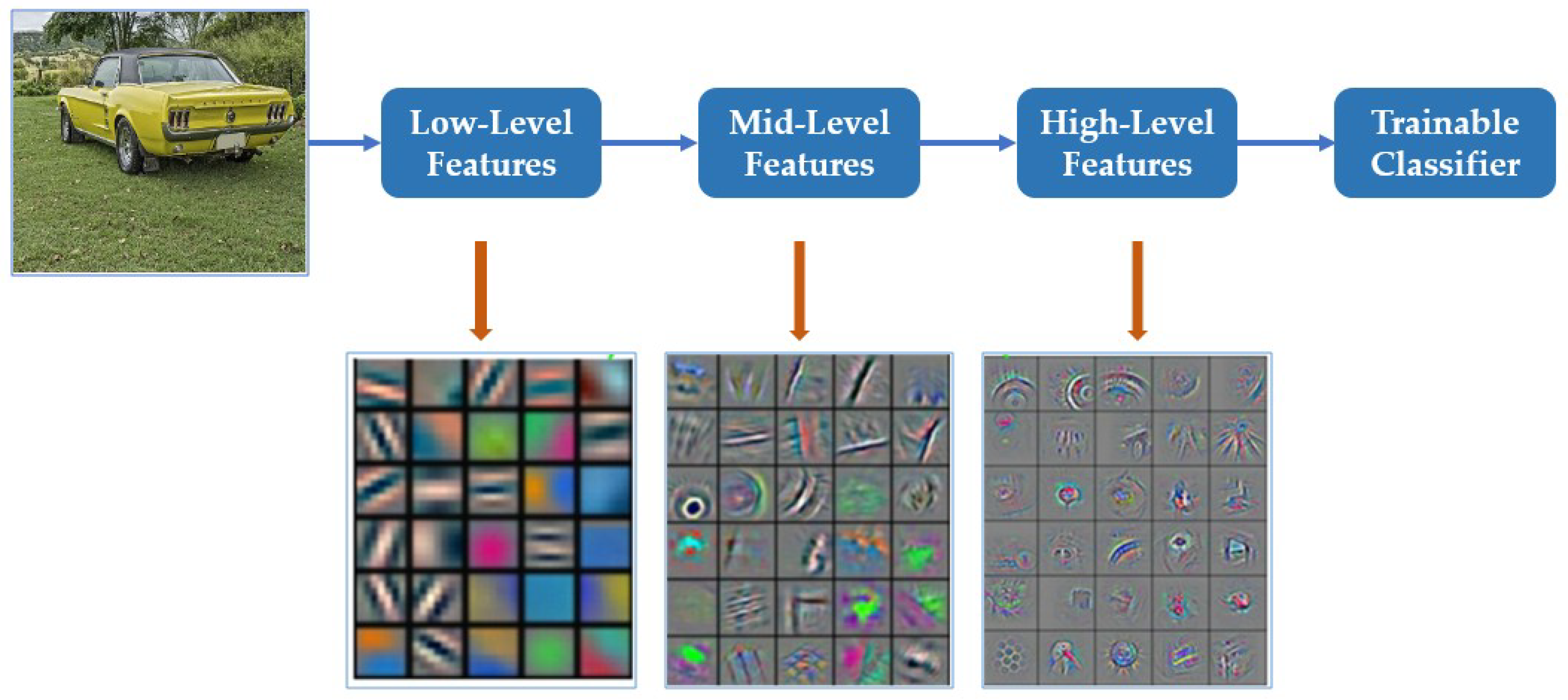
A variety of hardware and software techniques have been proposed to achieve energy and time efficiency [11,12,13,14]. One aspect involves reducing the testing complexity of the networks. Another focuses on reducing the training complexity of a CNN [15,16]. The latter is an important challenge for convolutional networks as high computational energy and time are needed. Especially in some online training applications in which the training time is included in the system action, reducing the training complexity means reducing the whole real-time action. At the same time, the dependence on platform can be reduced by the implementation of an energy-efficient network, which is important to some simple platforms. CNN-based feature extraction is a purely data-driven technique that can learn robust representations from data, but usually at the cost of high computational time and energy requirements [17]. Trainable random kernels in CNNs are adjusted to the appropriate value step-by-step through the continuous cycle iteration of samples to express the depth characters. Sufficient training data and iteration times demonstrated that the training of regular trainable weight kernels is a process that consumes considerable amounts of energy and time. Anisotropic filtering techniques have been widely used to extract robust image representations [18,19]. The optimization of anisotropic filters is much simpler. Anisotropic filters determined by a small part of samples can often effectively express the common features of all samples. Hence, the combination of CNNs with anisotropic filters is a valid process to reduce the computational energy and time consumption of networks. Among them, Gabor filters have attracted attention due to their ability to provide discriminative and informative features [20]. Compared with other filtering approaches, Gabor filters are advantageous in spatial information extraction, including edges and textures [21]. Through the deep convolution neural network visualization toolbox “Yo shin ski/Deep-Visualization-Toolbox” [22], we can obtain convolutional kernels for each level by visualizing a pretrained CNN model, as shown in Figure 1. The visualization of CNN kernels indicates that they are often redundant, and most of the convolutional kernels are similar to some structural Gabor filters. This similarity and the inherent error resiliency of the networks were the basis of incorporating Gabor kernels into CNNs.
Based on the inherent error resiliency of the networks and the similarity between convolutional kernels and Gabor filters, we introduced Gabor kernels into CNNs, and propose Gabor CNNs to reduce the computational energy and time required by networks, while maintaining a competitive output accuracy. In order to effectively imitate the structural characteristics of traditional weight kernels, we improved the two-dimensional Gabor filters by introducing parameters k1, k2, and k3 to adjust the oriented complex sinusoidal grating part. The improved Gabor filters have stronger frequency and orientation representations. We trained standard CNNs with a few samples and epochs as preliminary CNNs (or evaluation structures) to introduce and evaluate improved Gabor kernels in the first convolutional layer. To optimize the Gabor kernels in the first convolutional layer of preliminary CNNs, we designed a new multipopulation genetic algorithm (MPGA) [23,24] training method. In the iteration of MPGA, we optimized the Gabor kernels of the network by minifying global samples error, based on a small portion of samples and the structure of neural networks. Through the much simpler optimization of Gabor kernels, required computing resources were reduced, rather than using a purely data-driven method. Simultaneously, we created a procedure to train Gabor CNNs, termed the fast training method (FTM). In the FTM, we designed the Gabor convolutional layer of the network using MPGA based on a small portion of samples, but trained the remaining network structures using back-propagation [1] based on all samples. The FTM reasonably allocates the energy consumption of each layer of the network. Given the structure of Gabor CNNs and the MPGA training method, we eliminated a significant fraction of the computation-heavy components in the training process, thereby producing a considerable reduction in computational energy and time consumption required for training. The experimental results show that our proposed methodology is energy-efficient and reduces storage requirements and training time, with minimal degradation of the classification accuracy.
2. Related Work
2.1. Gabor Filters
After experiencing long-term evolution in nature, the biological vision system is one of the best information processing systems with the most complete mechanism. Riaz et al. used two-dimensional (2D) Gabor filters as a simple cell receptor field function to simulate its characteristics and responses [25,26]. A circular 2D Gabor filter is a combination of a 2D Gaussian function and an oriented complex sinusoidal grating. It is widely used to extract spatial local spectral features, which are important for multiple pattern recognition. Many previous works have attempted to extract important spatial information including edges and textures, with the advantage of Gabor filters in sparse representation. Gabor filters have been successfully applied to face recognition [27,28], fingerprint identification [29,30,31], and phase extraction [32] using Gabor atoms in sparse expression. A 2D Gabor filter as expressed as:
where , is a Gaussian envelope defined as:
where represents the coordinates of a pixel, , , denotes the standard deviation of a Gaussian envelope, denotes the wavelength of the span-limited sinusoidal grating, denotes the orientation in the interval , represents the aspect ratio of the space, and represents the phase shift. A 2D Gabor filter can be decomposed into a real part and an imaginary part , as shown in the following equations:
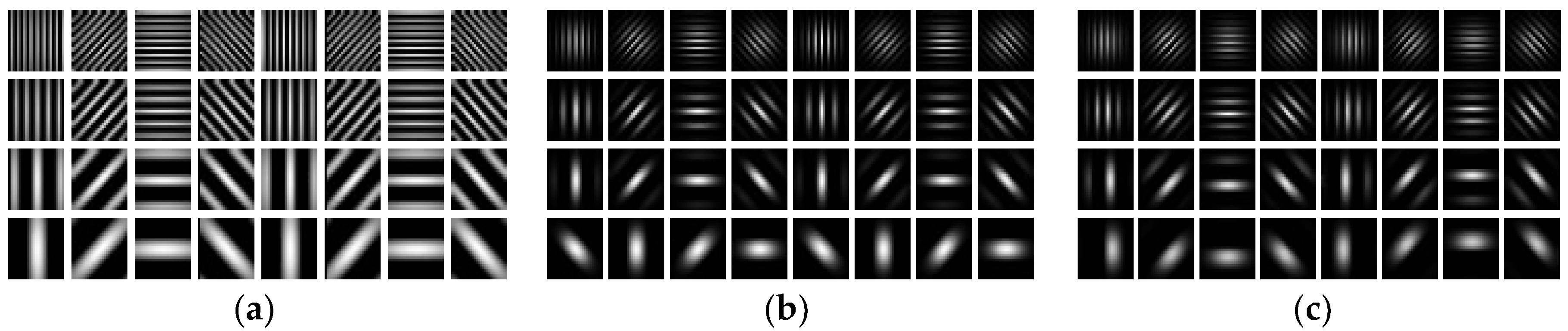
A circular 2D Gabor filter is a combination of a 2D Gaussian function and an oriented complex sinusoidal grating. The standard deviation of a Gaussian envelope controls the receptive field of Gabor filters. and control the wavelength and orientation of Gabor filters, respectively. The phase shift controls the distance between the center of the sinusoidal grating and the receptive field. Part of the traditional Gabor filters with different parameters are shown in Figure 2.
2.2. Convolutional Neural Network: Basics
The basic operation of CNNs consists of two stages: training and testing [33]. The testing process is basically forward propagation [34,35] and is used to test random data inputs, which is much simpler compared to training in terms of computational energy and time consumption. In the training process, a large number of samples are circularly iterated in CNNs, and random parameters are adjusted through gradient computation and weight update—both require considerable computation and time [16]. In this paper, we propose a method to achieve energy efficiency in training by removing a significant portion of the energy-hungry gradient computation and weight update operations with MPGA optimization.
CNNs consist of convolutional [36,37], pooling [36,37], and fully connected layers [38]. The nonlinear activation function [39,40] is applied at the end of the convolutional and fully connected layers. The convolutional layers are used to extract the depth features of the images [1,37]. The process is shown in Equation (5):
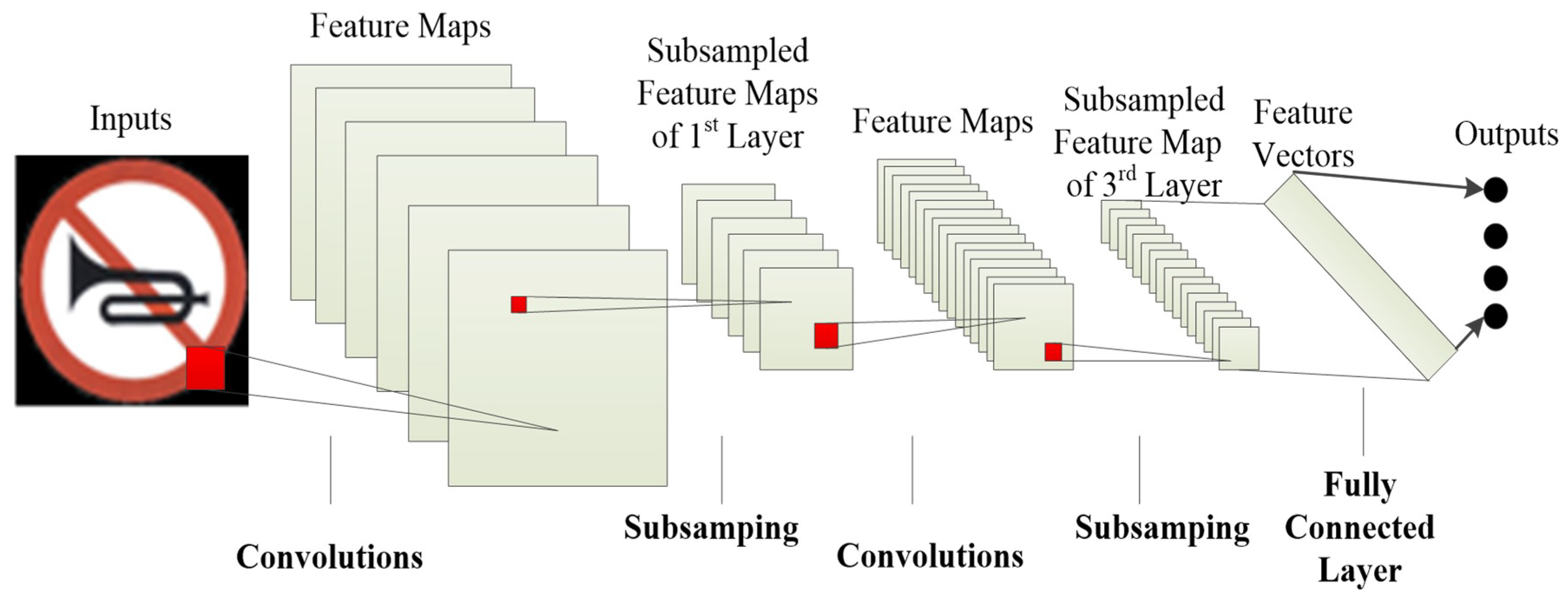
In Equation (5), is the input, is jth output feature map of the convolutional layer, indicates the nonlinear activation function, indicates the convolutional kernels of the convolutional layer, and represents the learnable bias added after the convolution operation before entering the activation function. indicates the operation of convolution. represents all feature maps in convolutional layer. Figure 3 represents a standard architecture of a deep-learning CNN.
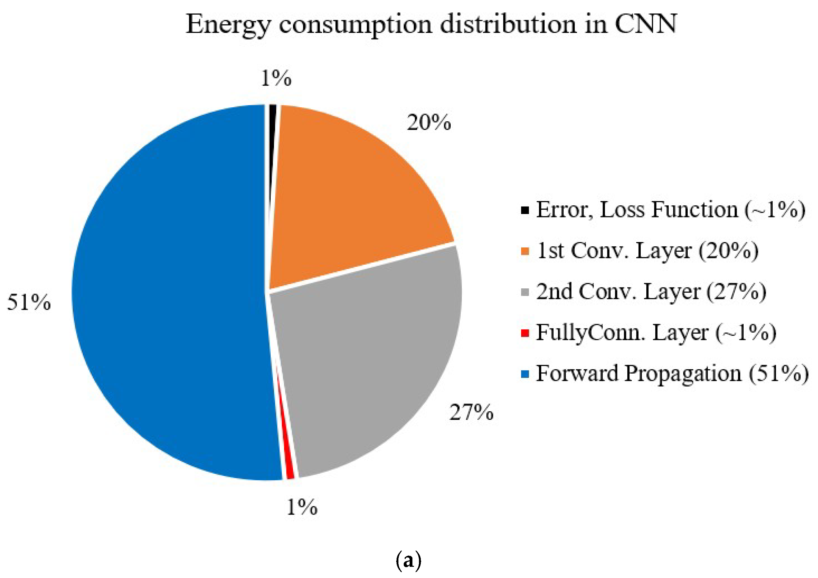
The main energy-hungry steps of CNN training (back-propagation) are gradient computation and the weight updates of the convolutional and fully connected layers. In Sarwar et al. [16], the authors proposed an energy model for quantifying the energy consumption of the network during training. In a conventional CNN denoted by [784 6c 2s 12c 2s 10o] (784 input neurons, 6 and 12 feature maps (6c and 12c) in the first and second convolutional layer, respectively, each followed by a pooling layer (2s) of stride 2, and finally, a fully connected output layer of 10 neurons, 10o), the second convolutional layer uses 27% of the overall energy consumption during training, whereas the first convolutional layer consumes 20%. In order to reduce computation and ensure network accuracy, we replaced trainable random kernels with Gabor filters. Because Gabor kernels do not require gradient computation and weight updates, the computation and time consumption of the Gabor convolutional layers are reduced.
2.3. Combination of Gabor Filters and CNNs
Studies have reported work undertaken to combine Gabor filters and CNNs. Such work can be divided into two main categories. In the first category, Gabor filters are used as a preprocessing step for neural network training to increase the accuracy of the networks, using the advantage of Gabor filters being similar to the simple human visual system [41,42] in the processes of texture feature expression and description [43]. In this method type, the optimization of Gabor filters usually adopts an empirical formula, which is not universal. In addition, this method increases the computational energy and time consumption with a preprocessing step. In the other category, Gabor filters are introduced into CNNs as Gabor kernels (or a Gabor convolutional layer) to eliminate the preprocessing step. In Chang et al. [15,44], the authors attempted to remove the preprocessing overhead by introducing Gabor filters into the first convolutional layer of a CNN. In Mahmoud et al. [44], Gabor filters were used to replace the random filter kernels in the first convolutional layer. The training was then limited to the remaining layers of the CNN. In Chang et al. [15], the Gabor kernels in the first layer were fine-tuned with training. In other words, the authors used Gabor filters as a good starting point for training the classifiers, which helps with convergence. In Sarwar et al. [16], Gabor filters were introduced in two convolutional layers. The authors discussed a scheme where Gabor filters are used to replace trainable random kernels in CNNs in order to decrease the computational energy and time consumption.
In the above studies, Gabor kernels were successfully introduced into the training process of CNNs, with less computational energy and time consumption. However, in the proposed methods, Gabor filters were used to replace convolutional kernels in pretrained CNNs, or to only selectively replace trainable kernels in CNNs, without training Gabor kernels in the convolutional layers of networks. Gabor kernels selected by empirical formula are always aiming at certain kinds of problems and may not match the network. In this work, we improved upon the traditional Gabor filters and designed a new MPGA training method to optimize them. Through the MPGA training method, our Gabor kernels become trainable in Gabor CNNs and more universal.
3. Proposed Method
3.1. Overview of Our Method
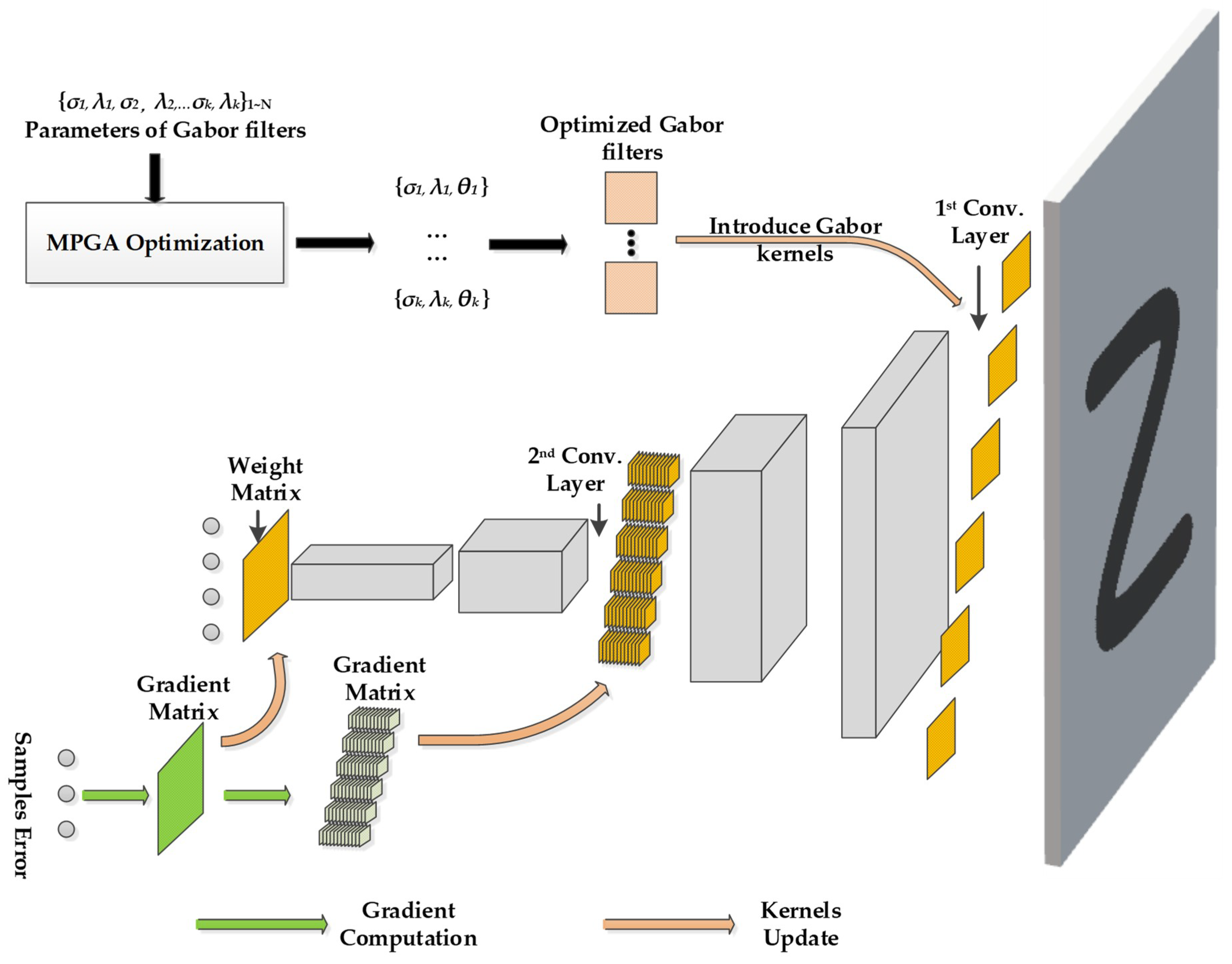
To address the computing-resource-saving problem, we develop Gabor convolutional neural network (Gabor CNN) and propose a fast training method (FTM) to train it. The structure of Gabor CNN and update of the convolutional layer and weight matrix in the fully connected layer is shown in Figure 5. The first convolutional layer of Gabor CNN consists of fixed Gabor kernels rather than trainable random weight matrix. In the FTM, the traditional Gabor filters are improved to imitate the structural characteristics of traditional weight kernels and introduced into the first convolutional layer. Then, we design a new training method based on the multipopulation genetic algorithm (MPGA) to optimize improved Gabor kernels instead of back-propagation. The training of Gabor kernels with MPGA is much more energy-efficient because less samples and iterations are needed. Finally, the rest of the Gabor CNN parameters are trained with back-propagation and all samples. The FTM for Gabor CNNs is shown in Figure 8. By replacing back-propagation with energy-efficient MPGA in the convolutional layer, we could eliminate a significant fraction of the computation-hungry components in the training process.
3.2. Improved Gabor Kernels in the First Convolutional Layer
For a given network, the size and number of trainable convolutional kernels are fixed. In order to maintain the accuracy and simultaneously reduce the computational energy and time consumption in the process of network training, we used Gabor kernels whose size and number were the same as regular trainable kernels, and whose orientations were equally spaced in direction and space to replace the kernels of the first layer of the CNN. In other words, the first layer of a Gabor CNN consists of Gabor kernels. With the introduction of Gabor filters with high-efficiency feature expression as convolutional kernels into CNNs, the feature extraction of the image can be expressed as:
The similarity between Gabor filters and convolutional kernels in the network and the inherent error resiliency of the networks are the basis of incorporating Gabor kernels into the proposed network. To enrich Gabor transformation, we introduced parameters to adjust the oriented complex sinusoidal grating part and defined the improved Gabor as:
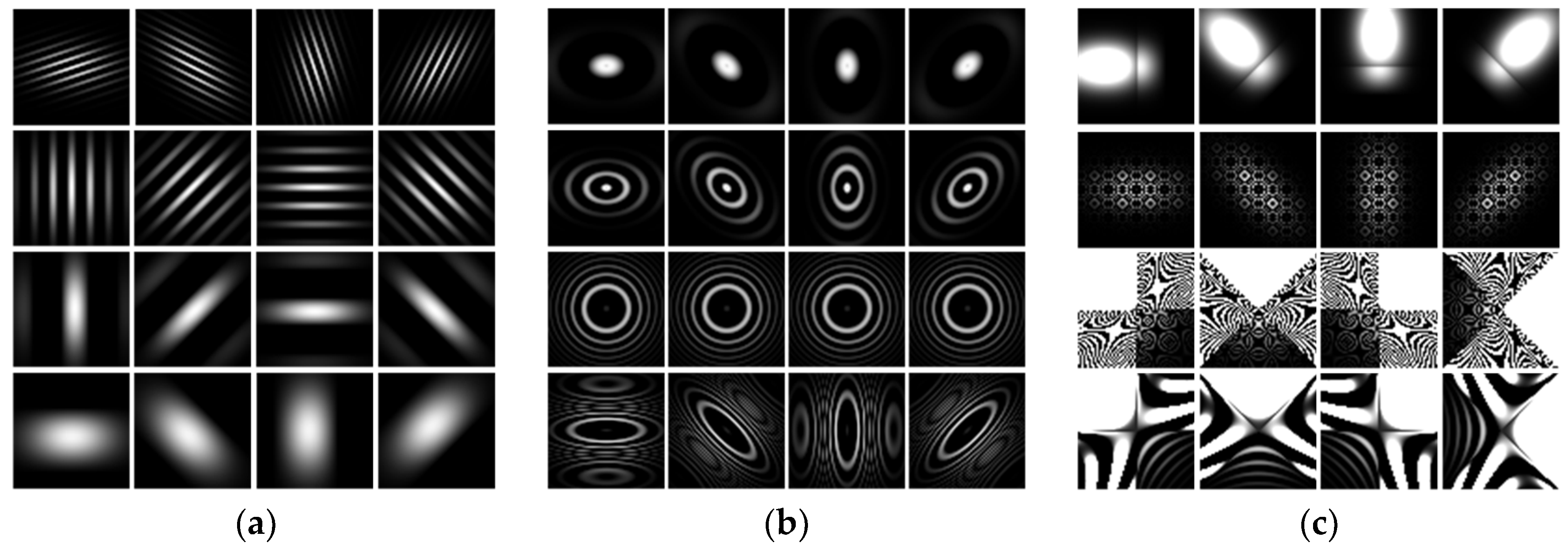
For example, for , the shape of Gabor filter is conventional with oriented grating; for , the Gabor filter is circular. Figure 4 shows part of the improved 2D Gabor filters.
In this paper, the Gabor CNN has two convolutional layers and each of them is followed by a subsampling layer. It has a fully connected layer that produces the final classification result. The first convolutional layer has k Gabor kernels, and the second convolutional layer extracts 2k features for each input with 2k random kernels. Taking the Mixed National Institute of Standards and Technology database (MNIST) [36] as an example, we used six Gabor kernels (with θ = 0°, 30°, 60°, 90°, 120°, and 150°) to form the first layer; hence, the second convolutional layer included 2k2 = 72 random kernels. The 12 feature maps from the second layer were used as feature vector inputs to the fully connected layer, which produced the final classification result. As a rule of thumb, we set the ratio of oriented, circular, and complicated Gabor kernels to 10:3:1.
To produce the predicted output, samples undergo forward propagation of a Gabor CNN—the same as the CNNs. However, the gradient computation and weight update are operated only at the fully connected and second convolutional layers. The Gabor kernels in the first convolutional layer are optimized by MPGA with minimal energy-consuming steps. Hence, in our proposed method, we achieve energy efficiency by eliminating a large portion of the gradient computation and weight update operations in the Gabor convolutional layer. In Figure 5, a schematic diagram shows an update of the convolutional layer and weight matrix in the fully connected layer in a Gabor CNN. Considering k = 6, there are six kernels in the first convolutional layer. Hence, the number of second convolutional layer kernels is 72, as mentioned above. In the Gabor CNN, the second convolutional layer and fully connected layer consist of trainable random kernels, but the first convolutional layer consists of optimized Gabor kernels. We trained standard CNNs with a few samples and epochs as preliminary CNNs (or evaluation structures) to introduce and evaluate improved Gabor kernels in the first convolutional layer. In order to select the most fitting Gabor kernels, training based on MPGA and preliminary CNNs is used to optimize the Gabor filters’ parameters. Then, Gabor filters are established with an optimal set of parameters and are defined as Gabor kernels and introduced into the first convolutional layer. To train other parameters, only the gradient matrix of the fully connected and second convolutional layers is calculated by back-propagation with sample error. After that, the weights update is performed with gradient matrix and fixed learning rate, the same as in a conventional CNN. During continuous training, the Gabor CNNs meet the accuracy requirements and achieve energy efficiency. The comparison between MPGA optimization and back-propagation in the first convolutional layer is described in the next chapter.
3.3. MPGA Optimization for Gabor Convolutional Kernels
The CNN classification accuracy is based on the efficient expression of input features, and improper substitution of Gabor kernels results in irreparable accuracy degradation. Therefore, the optimization of Gabor kernels is the key to Gabor CNN accuracy. Different from other methods, the optimization of Gabor kernels in a convolutional layer should be suitable for the network structure. In this paper, the number and size of Gabor kernels are determined by a given CNN; in terms of orientation, they are equally spaced. The standard deviation of the Gaussian envelope σ and the frequency of the span-limited sinusoidal grating μ cover the whole solution space. In order to select suitable Gabor kernels and produce a fast-learning first convolutional layer, we propose MPGA optimization for the standard deviation of a Gaussian envelope and the frequency of the span-limited sinusoidal grating.
A simple multipopulation genetic algorithm is an iterative procedure that maintains a constant-sized population (P) of candidate solutions consisting of individuals. During each generation, three genetic operators, called reproduction, crossover, and mutation, are performed to generate new populations. The best individual that represents the optimal solution in each generation is saved for the next generation. A cost function is used to evaluate the fitness values of individuals in each generation. An appropriate cost function is the key to MPGA optimization. The direction of error gradient descent in MPGA optimization for the Gabor convolutional layer must be the same as the direction of the error gradient descent in the training of CNNs. In this paper, we use global error as the cost function of MPGA optimization. The global error refers to the binomial norm of difference between the predicted values of all samples through CNNs and standard values, which is an important index that reflects the accuracy. In other words, the descent of global error can directly reflect the rise of network accuracy. The global error can be expressed as:
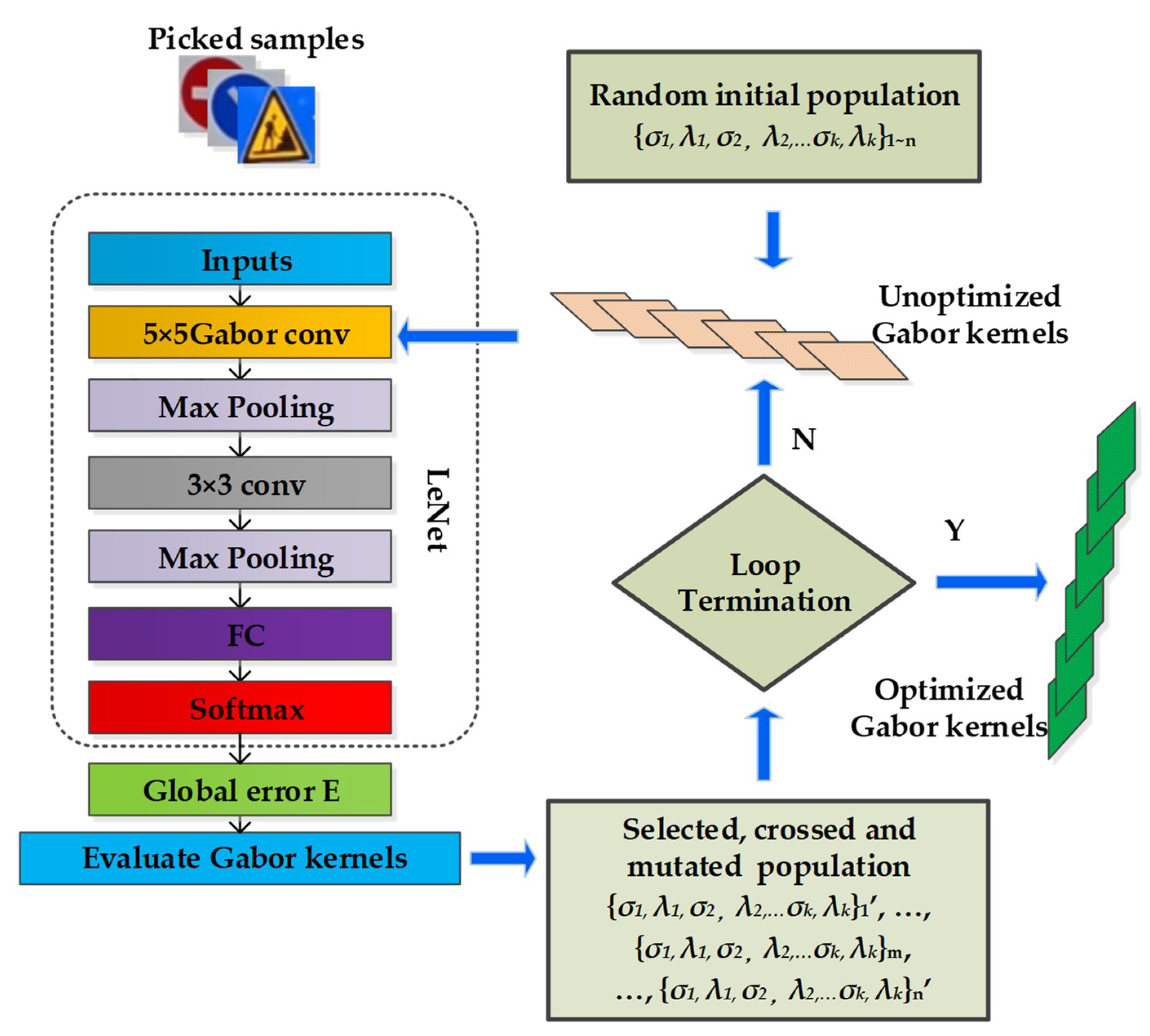
where is the predicted value of the kth sample through Gabor CNNs, is its label value, and n represents the number of samples. In this work, the global error was used as the cost function of MPGA optimization. Using the above description, MPGA optimization for Gabor convolutional kernels using the global error as the cost function can be expressed as shown in Figure 6.
The MPGA optimization for Gabor convolutional kernels is as follows:
- (1)
- An initial population P with a constant size 2k is randomly generated. k is the number of Gabor convolutional kernels in the first layer. Genes of individuals in the population represent the standard deviation of Gaussian envelope and the frequency of the span-limited sinusoidal grating of Gabor kernels.
- (2)
- The fitness for each initial individual corresponding to Gabor kernels is calculated.
- (3)
- The next generation, including the best individual from the previous generation, is created through reproduction, crossover, and mutation.
- (4)
- Each individual in the new generation is evaluated and the best Gabor kernels corresponding to one individual are saved.
- (5)
- If the search goal is achieved, or an allowable generation is attained, the best individual corresponding to Gabor kernels is returned as the solution; otherwise, return to step (3).
The training of improved Gabor kernels with MPGA is much more energy-efficient than the back-propagation method with a few samples and iterations. Some of the conventional trained kernels and optimized Gabor kernels of the first convolutional layer are shown in Figure 7.
3.4. Fast Training Method for Gabor Convolutional Neural Networks
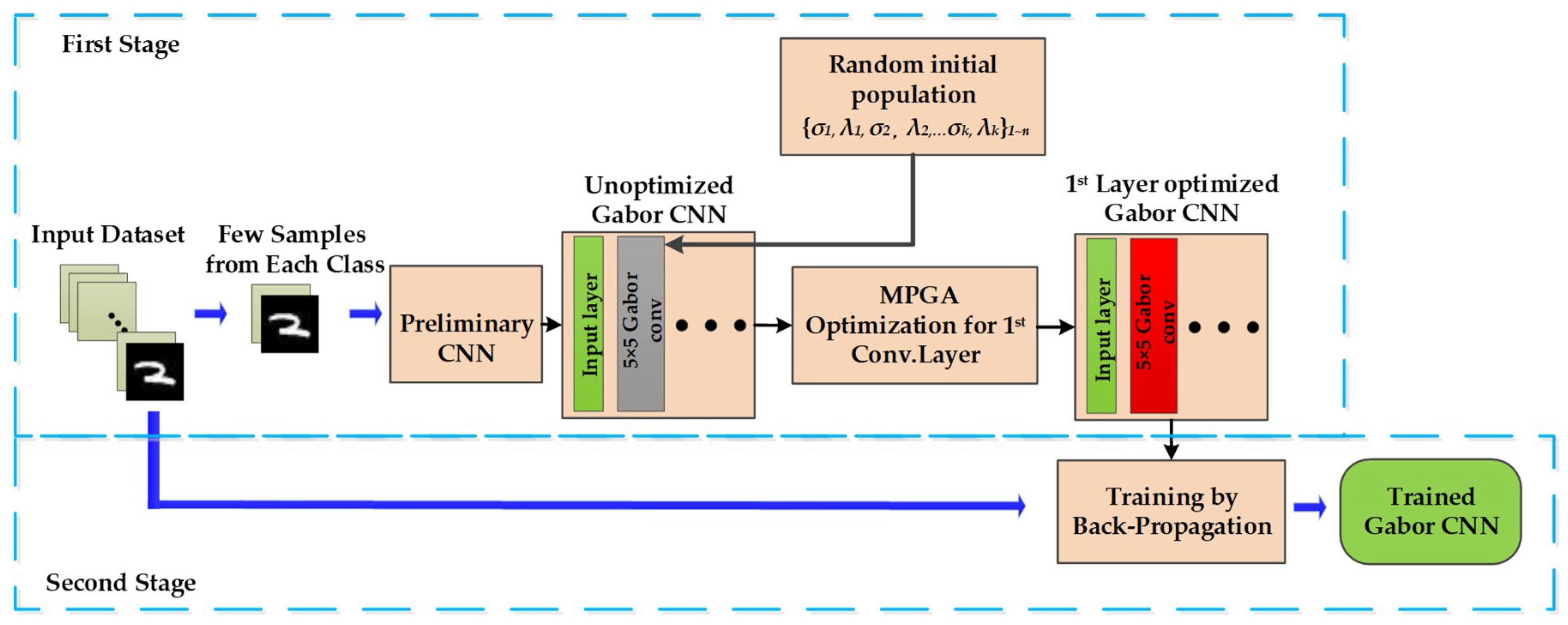
Trainable random kernels in CNNs are adjusted to the appropriate values by gradient computation and weight update, which are not fit for Gabor kernels. Different from other methods (such as the empirical formula), optimization of Gabor kernels in the convolutional layer should be suitable for the network structure. In this paper, we propose an FTM for Gabor CNNs. The Gabor convolutional layer is fast trained with MPGA and the evaluation structure, and then the rest of the Gabor CNN parameters are trained with back-propagation. The FTM for the Gabor CNNs is shown in Figure 8.
The basic operation of FTM consists of two stages: (1) optimization of Gabor convolutional kernels with a few samples and evaluation structure; and (2) training other Gabor CNNs parameters with all samples.
Gabor kernels can effectively express common features (like edges and texture) with simple optimization. Hence, we propose MPGA optimization with fewer iterations for the Gabor convolutional layer instead of training with a fixed learning rate. The Gabor features of the samples are similar within the same class but differ from those in other classes, which has been proven in many classification problems [32,44]. Based on the above reasoning, MPGA optimization for Gabor kernels can be completed with few representative samples. Degradation of the classification accuracy can be compensated for by the inherent error resiliency of the networks and the efficient ability to express Gabor kernels. In the first stage, a preliminary CNN is established with traditional randomly weighted kernels as the evaluation structure. Then, Gabor kernels constructed by a random initial population are incorporated into a preliminary CNN to replace the random kernels. An MPGA training method and a few samples from each class are used to optimize the Gabor convolutional layer and the output of the first layer of the optimized Gabor CNN. The training of improved Gabor kernels with MPGA is much more energy-efficient with fewer samples and iterations. In other words, we achieved energy efficiency by eliminating a large portion of the gradient computation and weight update operations in the first stage. In the second stage, other Gabor CNN parameters are trained with back-propagation to improve the network accuracy. The experiment results show that the inherent error resiliency of the networks and the ability of Gabor kernels to efficiently express features can effectively minimize the loss of accuracy.
4. Implementation and Experiment
In this section, we present the details of implementation of the Gabor CNN and the MGPA training method. We used modified versions of open-source MATLAB (MathWorks, Natick, MA, USA) codes [45,46] to implement multilayer CNNs for our experiments. We incorporated Gabor kernels into CNNs with MPGA optimization and the evaluation structure mentioned above to realize Gabor CNNs. Firstly, we used an example to analyze the energy efficiency and performance of Gabor CNNs on MINIST. Then, the accuracy, training time, and storage requirement were compared between two structures on the datasets listed in Table 1. We discussed the effects of iterations and the sampling rate in MPGA optimization on the three indicators above.
The architectures of two structures and parameters of MPGA optimization are listed in Table 2.
4.1. Energy Efficiency and Performance
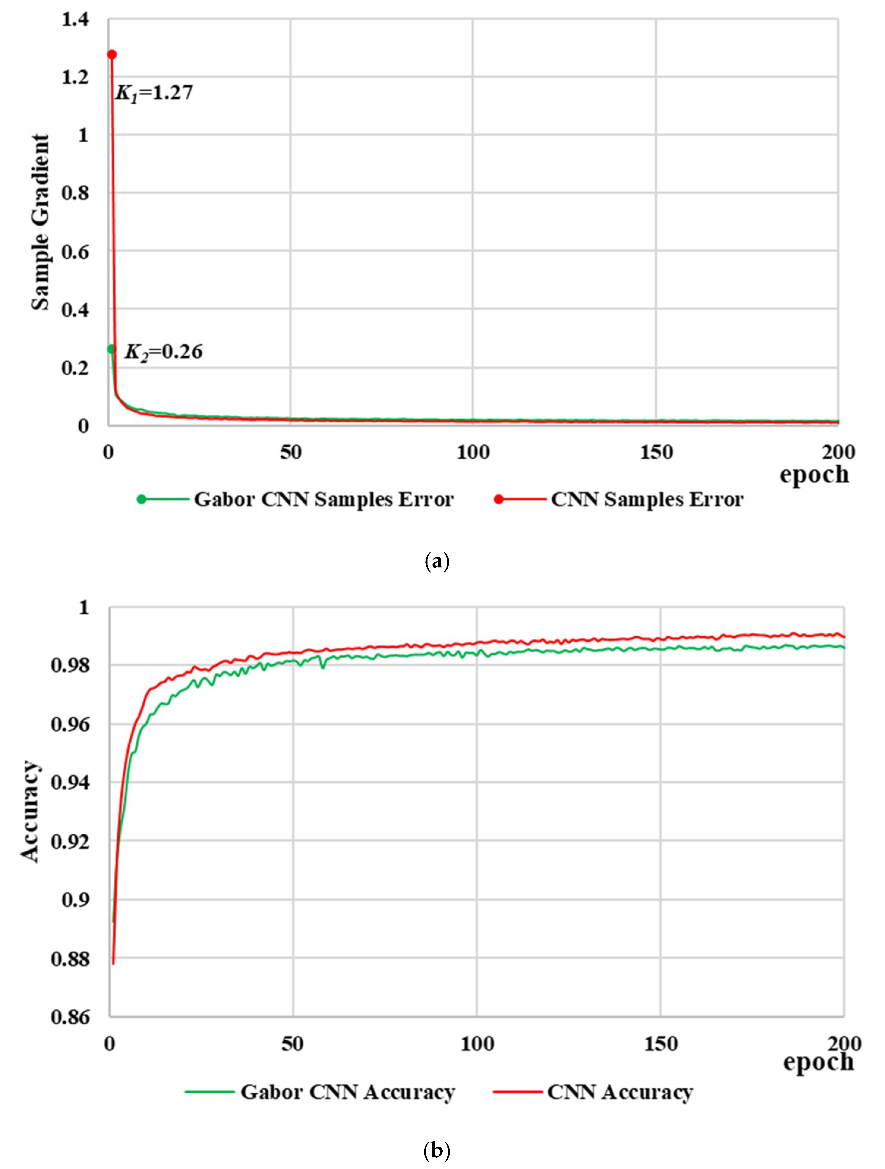
We conducted an experiment where we trained a CNN ([784 6c 2s 12c 2s 10o]) and a Gabor CNN with the same structure on the MINIST dataset. Each of the structures was trained for 200 epochs. Figure 9 shows the overall classification accuracy and mean square error obtained from each structure. In the plot (Figure 9a), the red curve corresponds to the CNN samples’ mean square error and the green curve corresponds to the Gabor CNN samples’ mean square error. K1 (1.27) and K2 (0.26) are the initial values of the samples’ mean square error of each structure. The difference between K1 and K2 indicates that optimized Gabor kernels can drastically reduce the samples’ mean square error and that the Gabor CNNs have preliminary identification ability. In the plot (Figure 9b), the red and green curves correspond to the overall classification accuracy of CNN and Gabor CNN, respectively. The degradation in classification accuracy is less than 1% and the curves in the two groups show similar trends. The trends in both curves suggest that CNN and Gabor perform similarly, but Gabor CNN is more efficient in terms of computing. As expected, incorporating Gabor kernels into CNNs causes minimal degradation in network performance, and MPGA optimization is a process that increases the overall classification accuracy.
Fewer training data were used and fewer iterations were required for the optimization of Gabor kernels than for the CNN training process. Hence, the energy consumption during the optimization of Gabor kernels is far less than in gradient computation and weight update of the first random convolutional layer with back-propagation. Convolution is the main operator in both MPGA optimization and back-propagation. In Table 3, the number of convolutions (Conv) operated in optimization of Gabor kernels and back-propagation (in standard CNN) method for one iteration in the forward process (FP) and back process (BP) of the first layer in both structures are listed for comparison. The optimization of Gabor kernels includes two parts: a preliminary CNN is established with randomly weighted kernels and MPGA for the first convolutional layer replaced by Gabor kernels. Correspondingly, the number Conv operated in optimization of Gabor kernels includes the number of Conv in both MPGA and the preliminary CNN.
The computational energy and time required for the optimization of Gabor kernels completes the genetic algorithm iterations and training for the preliminary CNN. Table 3 shows that the number of convolutions operated in MPGA for one iteration in the forward process (FP) and back process (BP) is more than in back-propagation. However, fewer iterations are needed in MPGA optimization than in the back-propagation method. It can be seen from the calculation that the computational energy consumption required for the optimization of Gabor kernels is 3–7% of the back-propagation in the conventional CNN. In Figure 10, the pie chart represents different computation distributions between Gabor and conventional CNNs across different segments. The energy of the error and loss function consumes a small fraction (~1%) in both structures. The energy consumption of the second convolutional layer and forward propagation in the two structures are the same in training. However, the energy consumption proportion of the first convolutional layer in Gabor CNN is about 1%, which is far less than in the conventional CNN. Of the entire 20% energy consumption required for the conventional CNN in the first convolutional layer, 19% of the energy can be saved by the optimized Gabor kernels in Gabor CNNs because Gabor kernels do not require gradient computation and weight update.
4.2. Accuracy Comparison
We trained two structures on datasets listed in Table 2 for 200 epochs to determine the accuracy, training time, and storage requirement information. The number of epochs was determined ensuring that all trainings converged and reached saturation. In each dataset, the Gabor CNN and conventional CNN had the same structure, and the latter was used as a baseline. The accuracies of networks are listed in Table 4.
Row 1 in Table 4 shows the accuracy of the two structures on MINIST. The accuracy decrease of the Gabor CNN is minimal. This result can be attributed to the fact that MINIST is a grayscale image dataset where edges and textures are remarkable features in the classification and the advantages of Gabor kernels in spatial information extraction can be fully reflected. However, the decreased accuracy of Gabor CNN in GTSRB is larger but tolerable. The larger accuracy loss may have occurred because the edges and textures are not all remarkable features in Traffic Sign Recognition, considering color is prominent in some situations. In Face Recognition, the accuracy of Gabor CNN is better than that at baseline. As ORL has fewer samples, and MPGA optimization for Gabor kernels can overcome this problem, this may be the reason for better accuracy.
4.3. Training Time Comparison
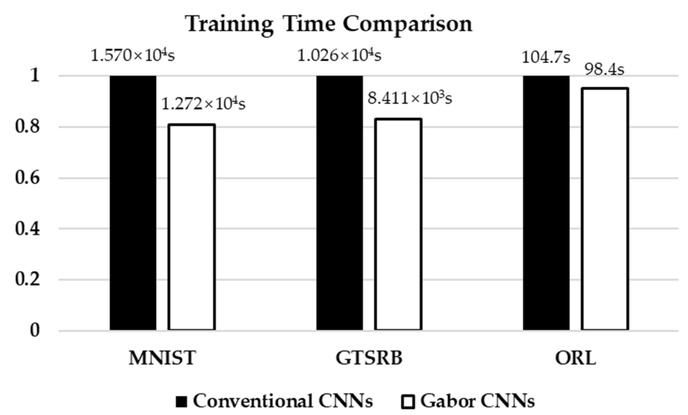
The bar chart in Figure 11 shows the normalized training time after 200 epochs of the two structures in each dataset. The training time of conventional CNN in three datasets is about 1.570 × 10⁴ s, 1.026 × 10⁴ s, and 104.7 s, respectively. Correspondingly, the training time of our Gabor CNN is about 1.272 × 10⁴ s, 8.411 × 10³ s, and 98.4 s. Since FTM involves optimization of Gabor convolutional kernels and training other parameters, the Gabor CNN training time includes the corresponding two parts. Less training data and iterations are required for optimization of Gabor kernels compared to the training process of CNN. Hence, considerably less training time is required for the optimization of Gabor kernels than for the gradient computation and weight update of the first random convolutional layer with back-propagation. We observed a 17–19% reduction in training time in MINIST and GTSRB. However, this reduction was not obvious in ORL as ORL had fewer samples and we must increase the sampling rate of MPGA optimization to ensure that the Gabor convolutional kernels are optimized. In conclusion, we achieved a significant reduction in training time with sufficient samples.
4.4. Storage Requirement Comparison
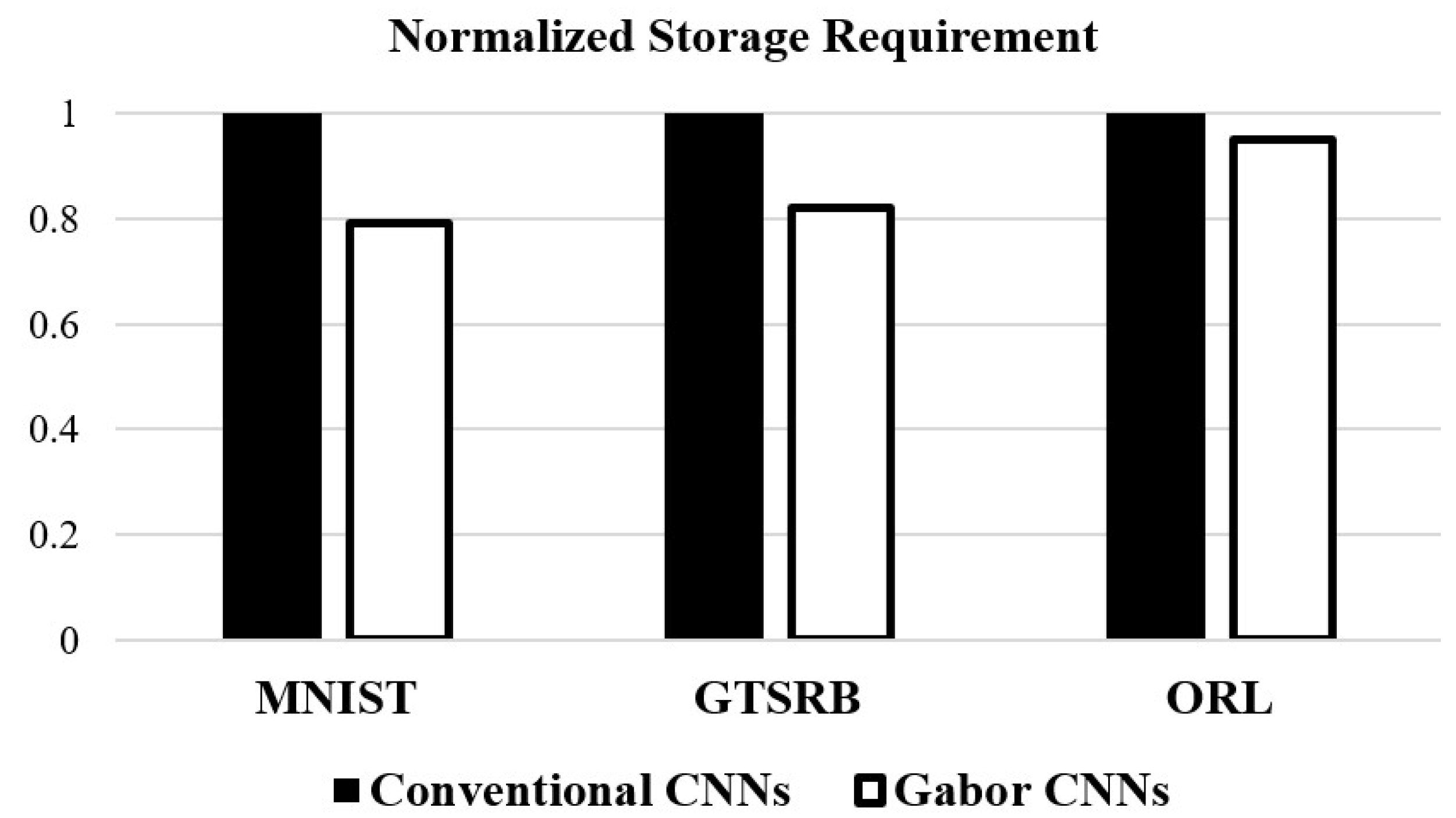
Figure 12 shows the storage requirement reduction obtained using the proposed scheme for different applications. We achieved a 6–21% reduction in storage requirements across the various benchmarks for the memory read/write operations. The reduction was not obvious in ORL as ORL had fewer samples and the computation saved by MPGA optimization is not obvious. In forward propagation, each kernel requires one read operation, and in back-propagation, each kernel requires one write operation. We observed an 18–21% reduction in the storage requirements in MINIST and GTSRB. The proposed Gabor CNNs and FTM significantly improved in storage requirements with sufficient samples.
4.5. Effects of Iterations and Sampling Rate
The Gabor convolutional layer was trained with MPGA and the evaluation structure. The iterations and the sampling rate are key parameters of MPGA optimization. Insufficient iterations and sampling rate could cause the improper substitution of Gabor kernels, resulting in irreparable accuracy degradation. Conversely, superfluous iterations or sampling rate minimize the reduction in training time and storage requirements. The line chart in Figure 13a shows the training time reductions of different iterations and sampling rates in MNIST. With increasing iterations and sampling rate, the training time reduction decreased correspondingly. In Figure 13b, the accuracy was maximized when the number of iterations was about 20 and the sampling rate was about 0.1. The results show the significant negative linear correlation between the training time reduction and the sampling rate. The accuracy was the highest value when the sampling rate was over 1%. To obtain the greatest degree of training time reduction, we set the sampling rate to 1% and the number of iterations to 20 in MINIST.
5. Conclusions
High computational energy and the time required hinder the practical application of CNNs. Due to the advantages of Gabor filters in spatial information extraction, including edges and textures, the combination of CNN with Gabor kernels efficiently reduces the training time and energy consumed. We improved the traditional Gabor filters by strengthening the frequency and orientation representations. Then, we introduced Gabor kernels into CNNs and termed it the Gabor Convolutional Neural Network (Gabor CNN) and designed a new training method based on the multipopulation genetic algorithm (MPGA) to optimize the improved Gabor kernels. We proposed a procedure to train Gabor CNNs, termed FTM. We eliminated a significant fraction of the energy-consuming components of back-propagation in the training process, thereby considerably reducing the energy and time consumption. In FTM, the Gabor convolutional layer was fast trained with MPGA and an evaluation structure, and then the remaining Gabor CNN parameters were trained with back-propagation. Experiments across various benchmark applications with our proposed scheme showed that Gabor CNNs and the MPGA training method reduced computational energy and time by 17–19% and storage requirements by 18–21% with a less than 1% accuracy decrease when samples were sufficient. However, the reduction of computational time and storage requirements are not obvious when sufficient samples are unavailable. Introducing Gabor filters into deeper layers is also difficult because the deeper convolutional layer is complex and the similarity between pretrained deep convolutional kernels and Gabor filters is poor. The accuracy of the network is difficult to guarantee when replacing all convolutional layers. Employing Gabor kernels is also beneficial for larger and more complex CNNs, considering the structure of Gabor CNNs and FTM. In the future, we will introduce Gabor kernels into more complicated CNNs and applications.
Author Contributions
F.M. and X.W. were responsible for the overall work and proposed the idea and experiments of the method in the paper, and the paper was written mainly by the two authors. F.S. performed part of the experiments and contributed to many effective discussions in both ideas and writing. D.W. provided many positive suggestions and comments for the paper. X.H. performed part of the experiments and provided many good suggestions.
Funding
This work was supported by the National Key Research and Development Program of China under grant 2016YFC0802904, National Natural Science Foundation of China under grant 61671470, and the Postdoctoral Science Foundation Funded Project of China under grant 2017M623423.
Conflicts of Interest
The authors declare no conflict of interest.
References
- Tom, Y.; Devamanyu, H.; Soujanya, P.; Erik, C. Recent trends in deep learning based natural language processing. IEEE Comput. Intell. Mag. 2018, 13, 55–75. [Google Scholar] [CrossRef]
- Marcus, G. Deep Learning: A Critical Appraisal. arXiv, 2018; arXiv:1801.00631. [Google Scholar]
- Han, J.; Zhang, D.; Cheng, G.; Liu, N.; Xu, D. Advanced deep-learning techniques for salient and category-specific object detection: A survey. IEEE Signal Process. Mag. 2018, 35, 84–100. [Google Scholar] [CrossRef]
- Asif, U.; Bennamoun, M.; Sohel, F. A multi-modal, discriminative and spatially invariant CNN for RGB-D object labeling. IEEE Trans. Pattern Anal. Mach. Intell. 2017, 40, 2051–2065. [Google Scholar] [CrossRef]
- Chin, T.W.; Yu, C.L.; Halpern, M.; Genc, H.; Tsao, S.L.; Reddi, V.J. Domain-Specific Approximation for Object Detection. IEEE Micro 2018, 38, 31–40. [Google Scholar] [CrossRef]
- Ranjan, R.; Sankaranarayanan, S.; Bansal, A.; Bodla, N.; Chen, J.-C.; Patel, V.M.; Castillo, C.D.; Chellappa, R. Deep learning for understanding faces: Machines may be just as good, or better, than humans. IEEE Signal Process. Mag. 2018, 35, 66–83. [Google Scholar] [CrossRef]
- Ledig, C.; Theis, L.; Huszar, F.; Caballero, J.; Cunningham, A.; Acosta, A.; Aitken, A.; Tejani, A.; Totz, J.; Wang, Z.; et al. Photo-realistic single image super-resolution using a generative adversarial network. In Proceedings of the IEEE Conference on Computer Vision and Pattern Recognition (CVPR) 2017, Honolulu, HI, USA, 21–26 July 2017. [Google Scholar] [CrossRef]
- LeCun, Y.; Boser, B.; Denker, J.S.; Henderson, D.; Howard, R.E.; Hubbard, W.; Jackel, L.D. Backpropagation applied to handwritten zip code recognition. Neural Comput. 2014, 1, 541–551. [Google Scholar] [CrossRef]
- Hariharan, B.; Arbelaez, P.; Girshick, R.; Malik, J. Object instance segmentation and fine-grained localization using hypercolumns. IEEE Trans. Pattern Anal. Mach. Intell. 2017, 39, 627–639. [Google Scholar] [CrossRef]
- Wang, J.; Ma, Y.; Zhang, L.; Gao, R.X.; Wu, D. Deep learning for smart manufacturing: Methods and applications. J. Manuf. Syst. 2018, 48, 144–156. [Google Scholar] [CrossRef]
- Deng, L.; Yu, D. Deep learning: Methods and applications. Found. Trends Signal Process. 2014, 7, 197–387. [Google Scholar] [CrossRef]
- Li, H.; Fan, X.; Li, J.; Wei, C.; Zhou, X.; Wang, L. A high performance FPGA-based accelerator for large-scale Convolutional Neural Networks. In Proceedings of the International Conference on Field Programmable Logic & Applications, Lausanne, Switzerland, 29 August–2 September 2016. [Google Scholar] [CrossRef]
- Li, C.; Yang, Y.; Feng, M.; Srimat, C.; Zhou, H. Optimizing Memory Efficiency for Deep Convolutional Neural Networks on GPUs. In Proceedings of the International Conference for High Performance Computing, Networking, Storage & Analysis, Denver, CO, USA, 12–17 November 2017. [Google Scholar] [CrossRef]
- Ciresan, D.C.; Meier, U.; Masci, J.; Gambardella, L.M.; Schmidhuber, J. Flexible, High Performance Convolutional Neural Networks for Image Classification. In Proceedings of the International Joint Conference on IJCAI, Barcelona, Spain, 16–22 July 2011. [Google Scholar] [CrossRef]
- Chang, S.Y.; Morgan, N. Robust CNN-based speech recognition with Gabor filter kernels. In Proceedings of the Annual Conference of the International Speech Communication Association, Singapore, 14–18 September 2014; pp. 905–909. [Google Scholar]
- Sarwar, S.S.; Panda, P.; Roy, K. Gabor filter assisted energy efficient fast learning Convolutional Neural Networks. In Proceedings of the IEEE/ACM International Symposium on Low Power Electronics and Design, Taipei, Taiwan, 24–26 July 2017. [Google Scholar] [CrossRef]
- Chetlur, S.; Woolley, C.; Vandermersch, P.; Cohen, J.; Tran, J.; Catanzaro, B.; Shelhamer, E. Cudnn: Efficient primitives for deep learning. Comput. Sci. 2014. [Google Scholar] [CrossRef]
- He, L.; Li, J.; Plaza, A.; Li, Y. Discriminative low-rank gabor filtering for spectral-spatial hyperspectral image classification. IEEE Trans. Geosci. Remote Sens. 2017, 55, 1381–1395. [Google Scholar] [CrossRef]
- Rossovskii, L.E. Image filtering with the use of anisotropic diffusion. Comput. Math. Math. Phys. 2017, 57, 401–408. [Google Scholar] [CrossRef]
- Bovik, A.C.; Clark, M.; Geisler, W.S. Multichannel texture analysis using localized spatial filters. IEEE Trans. Pattern Anal. Mach. Intell. 2002, 12, 55–73. [Google Scholar] [CrossRef]
- Randen, T.; Husoy, J.H. Filtering for texture classification: A comparative study. IEEE Trans Pattern Anal. Mach. Intell. 1999, 21, 291–310. [Google Scholar] [CrossRef]
- Zeiler, M.D.; Fergus, R. Visualizing and Understanding Convolutional Networks. In Computer Vision—ECCV 2014; Springer: New York, NY, USA, 2014; pp. 818–833. [Google Scholar]
- Madhavi, D.; Ramesh Patnaik, M. Genetic Algorithm-Based Optimized Gabor Filters for Content-Based Image Retrieval. In Intelligent Communication, Control and Devices. Advances in Intelligent Systems and Computing, 2nd ed.; Singh, R., Choudhury, S., Gehlot, A., Eds.; Springer: Singapore, 2018; Volume 624, pp. 157–164. ISBN 978-981-10-5902-5. [Google Scholar]
- Ghodrati, H.; Dehghani, M.J.; Danyali, H. Iris feature extraction using optimized Gabor wavelet based on multi objective genetic algorithm. In Proceedings of the International Symposium on Innovations in Intelligent Systems and Applications, Istanbul, Turkey, 15–18 June 2011; pp. 159–163. [Google Scholar] [CrossRef]
- Riaz, F.; Hassan, A.; Rehman, S.; Qamar, U. Texture classification using rotation- and scale-invariant gabor texture features. IEEE Signal Process. Lett. 2013, 20, 607–610. [Google Scholar] [CrossRef]
- Tao, L.; Hu, G.H.; Kwan, H.K. Multiwindow real-valued discrete gabor transform and its fast algorithms. IEEE Trans. Signal Process. 2015, 63, 5513–5524. [Google Scholar] [CrossRef]
- Bhattacharya, S.; Dasgupta, A.; Routray, A. Robust face recognition of inferior quality images using Local Gabor Phase Quantization. Technol. Symp. 2017. [Google Scholar] [CrossRef]
- Li, C.; Wei, W.; Li, J.; Song, W. A cloud-based monitoring system via face recognition using gabor and cs-lbp features. J. Supercomput. 2017, 73, 1532–1546. [Google Scholar] [CrossRef]
- Kaggwa, F.; Ngubiri, J.; Tushabe, F. Combined feature level and score level fusion Gabor filter-based multiple enrollment fingerprint recognition. In Proceedings of the International Conference on Signal Processing, Auckland, New Zealand, 27–30 November 2017. [Google Scholar] [CrossRef]
- Fei, L.; Teng, S.; Wu, J.; Rida, I. Enhanced minutiae extraction for high-resolution palmprint recognition. Int. J. Image Graph. 2017, 17, 1750020. [Google Scholar] [CrossRef]
- Kumari, P.A.; Suma, G.J. An experimental study of feature reduction using PCA in multi-biometric systems based on feature level fusion. In Proceedings of the International Conference on Advances in Electrical, Putrajaya, Malaysia, 28–30 September 2017. [Google Scholar] [CrossRef]
- Jia, S.; Shen, L.; Zhu, J.; Li, Q. A 3-D gabor phase-based coding and matching framework for hyperspectral imagery classification. IEEE Trans. Cybern. 2017, 48, 1176–1188. [Google Scholar] [CrossRef] [PubMed]
- Bengio, Y. Learning deep architectures for AI. Found. Trends Mach. Learn. 2009, 2, 1–127. [Google Scholar] [CrossRef]
- Li, D. A tutorial survey of architectures, algorithms, and applications for deep learning. APSIPA Trans. Signal Inf. Process. 2014, 3, 1–29. [Google Scholar] [CrossRef]
- Palm, R.B. Prediction as a Candidate for Learning Deep Hierarchical Models of Data; Technical University of Denmark: Lyngby, Denmark, 2012. [Google Scholar]
- Lecun, Y.; Bottou, L.; Bengio, Y.; Haffner, P. Gradient-based learning applied to document recognition. Proc. IEEE 1998, 86, 2278–2324. [Google Scholar] [CrossRef] [Green Version]
- Lecun, Y.; Bengio, Y.; Hinton, G. Deep learning. Nature 2015, 521, 436–444. [Google Scholar] [CrossRef] [PubMed]
- Krizhevsky, A.; Sutskever, I.; Hinton, G. Imagenet classification with deep Convolutional Neural Networks. In Proceedings of the International Conference on Neural Information Processing Systems, Lake Tahoe, NV, USA, 3–6 December 2012; pp. 1097–1105. [Google Scholar] [CrossRef]
- He, K.; Zhang, X.; Ren, S.; Sun, J. Deep residual learning for image recognition. In Proceedings of the IEEE Conference on Computer Vision and Pattern Recognition (CVPR), Las Vegas, NV, USA, 26 June–1 July 2016. [Google Scholar] [CrossRef]
- Yeo, I.; Gi, S.G.; Lee, B.G.; Chu, M. Stochastic implementation of the activation function for artificial neural networks. In Proceedings of the Biomedical Circuits & Systems Conference, Torino, Italy, 19–21 October 2017. [Google Scholar] [CrossRef]
- Hubel, D.H.; Wiesel, T.N. Receptive fields of single neurons in the cat’s striate cortex. J. Physiol. 1959, 148, 574–591. [Google Scholar] [CrossRef] [PubMed]
- Hubel, D.H.; Wiesel, T.N. Receptive fields, binocular interaction and functional architecture in the cat’s visual cortex. J. Physiol. 1962, 160, 106–154. [Google Scholar] [CrossRef]
- Chen, Y.; Zhu, L.; Ghamisi, P.; Jia, X.; Li, G.; Tang, L. Hyperspectral images classification with gabor filtering and Convolutional Neural Network. IEEE Geosci. Remote Sens. Lett. 2017, 14, 2355–2359. [Google Scholar] [CrossRef]
- Mahmoud, S.A. Arabic (Indian) handwritten digits recognition using Gabor-based features. In Proceedings of the International Conference on Innovations in Information Technology, Al-Ain, Abu Dhabi, 15–17 December 2009. [Google Scholar] [CrossRef]
- Palm, R.B. MATLAB/Octave Toolbox for Deep Learning. Available online: https://github.com/rasmusbergpalm/DeepLearnToolbox/ (accessed on 1 December 2015).
- Vedaldi, A.; Lenc, K. MatConvNet: Convolutional Neural Networks for MATLAB. In Proceedings of the 23rd Annual ACM Conference on Multimedia, Brisbane, Australia, 26–30 October 2015; pp. 689–692. [Google Scholar] [CrossRef]
Figure 1.
Convolutional kernels of each level by visualizing a pretrained convolutional neural network (CNN) model.
Figure 1.
Convolutional kernels of each level by visualizing a pretrained convolutional neural network (CNN) model.

Figure 2.
Part of traditional Gabor filters with different parameters: (a) , (from left to right), (from top to bottom), and ; (b) , (from left to right), (from top to bottom), and ; (c) , (from left to right), (from top to bottom), and .
Figure 2.
Part of traditional Gabor filters with different parameters: (a) , (from left to right), (from top to bottom), and ; (b) , (from left to right), (from top to bottom), and ; (c) , (from left to right), (from top to bottom), and .

Figure 3.
A standard architecture of a deep-learning Convolutional Neural Network (CNN).

Figure 4.
Improved two-dimensional (2D) Gabor filters with various shapes: (a) Conventional Gabor filters with oriented grating, (b) circular Gabor filters, and (c) more complicated Gabor filters.
Figure 4.
Improved two-dimensional (2D) Gabor filters with various shapes: (a) Conventional Gabor filters with oriented grating, (b) circular Gabor filters, and (c) more complicated Gabor filters.

Figure 5.
Update of convolutional layer and weight matrix in the fully connected layer in a Gabor CNN.
Figure 5.
Update of convolutional layer and weight matrix in the fully connected layer in a Gabor CNN.

Figure 6.
Flow chart of multipopulation genetic algorithm (MPGA) optimization for Gabor convolutional kernels. Individual represents a combination of Gabor kernels in the convolutional layer. The individual is the optional individual selected from the previous generation.
Figure 6.
Flow chart of multipopulation genetic algorithm (MPGA) optimization for Gabor convolutional kernels. Individual represents a combination of Gabor kernels in the convolutional layer. The individual is the optional individual selected from the previous generation.

Figure 7.
(a) Visualization of part of the conventional trained kernels and (b) optimized Gabor kernels of the first convolutional layer (with θ = 0°, 30°, 60°, 90°, 120°, and 150°).
Figure 7.
(a) Visualization of part of the conventional trained kernels and (b) optimized Gabor kernels of the first convolutional layer (with θ = 0°, 30°, 60°, 90°, 120°, and 150°).

Figure 8.
Fast training method for Gabor CNNs.

Figure 9.
(a) Samples’ mean square error and (b) overall classification accuracy obtained from each structure.
Figure 9.
(a) Samples’ mean square error and (b) overall classification accuracy obtained from each structure.

Figure 10.
Energy consumption distribution: (a) conventional CNN and (b) Gabor CNN on MINIST.


Figure 11.
The normalized training time after 200 epochs of the two structures in each dataset.

Figure 12.
The normalized storage requirement reduction of the two structures in each dataset.

Figure 13.
(a) Training time reduction and (b) accuracy with different numbers of iterations and different sampling rates in MNIST.
Figure 13.
(a) Training time reduction and (b) accuracy with different numbers of iterations and different sampling rates in MNIST.


Table 1.
Benchmarks used in experiments.
| Application | Dataset | No. Training Samples | No. Testing Samples | Input Image Size |
|---|---|---|---|---|
| Digit Recognition | MNIST | 60,000 | 10,000 | 28 × 28 |
| Traffic Sign Recognition | GTSRB | 39,200 | 5000 | 32 × 32 (Normalized) |
| Face Recognition | ORL | 400 | 200 | 92 × 112 |
Table 2.
Architectures of two structures and parameters of MPGA optimization.
| Dataset | Network | Population & Individual | Crossover & Mutation | Sampling Rate |
|---|---|---|---|---|
| MNIST | [784 (5 × 5)6c 2s (5 × 5)12c 2s 10o] | 50 12 | 0.8 0.6 | 1% |
| GTSRB | [1024 (5 × 5)8c 2s (5 × 5)12c 2s 42o] | 50 16 | 0.8 0.6 | 1% |
| ORL | [4096 (11 × 11)8c 2s (5 × 5)12c 2s 40o] | 10 16 | 0.2 0.4 | 10% |
Table 3.
Convolutions used in MPGA optimization and back-propagation in the first layer.
| Method | Conv in FP | Conv in BP | Iterations | All Conv |
|---|---|---|---|---|
| MPGA | 1.8 × 10⁵ | -- | 10 | 1.8 × 10⁶ |
| Preliminary CNN | 4.7 × 10⁴ | 4.7 × 10⁴ | 10 | 9.4 × 10⁵ |
| Back-propagation | 3.6 × 10⁵ | 3.6 × 10⁵ | 200–500 | 1.5–3.6 × 10⁸ |
Preliminary CNN (or evaluation structure) and conventional CNN denoted by [784 6c 2s 12c2s 10o] In MPGA optimization, the sampling rate is 1%, the population number is 50, and the number of genetic iterations is 10.
Table 4.
Accuracies of networks.
| Dataset | Conventional CNN | Gabor CNN | Accuracy Change |
|---|---|---|---|
| MNIST | 99.11% | 98.66% | 0.45% |
| GTSRB | 98.70% | 96.24% | 2.46% |
| ORL | 98.60% | 99.10% | −0.50% |
© 2019 by the authors. Licensee MDPI, Basel, Switzerland. This article is an open access article distributed under the terms and conditions of the Creative Commons Attribution (CC BY) license (http://creativecommons.org/licenses/by/4.0/).
Share and Cite
MDPI and ACS Style
Meng, F.; Wang, X.; Shao, F.; Wang, D.; Hua, X. Energy-Efficient Gabor Kernels in Neural Networks with Genetic Algorithm Training Method. Electronics 2019, 8, 105. https://doi.org/10.3390/electronics8010105
AMA Style
Meng F, Wang X, Shao F, Wang D, Hua X. Energy-Efficient Gabor Kernels in Neural Networks with Genetic Algorithm Training Method. Electronics. 2019; 8(1):105. https://doi.org/10.3390/electronics8010105
Chicago/Turabian StyleMeng, Fanjie, Xinqing Wang, Faming Shao, Dong Wang, and Xia Hua. 2019. "Energy-Efficient Gabor Kernels in Neural Networks with Genetic Algorithm Training Method" Electronics 8, no. 1: 105. https://doi.org/10.3390/electronics8010105
Note that from the first issue of 2016, this journal uses article numbers instead of page numbers. See further details here.