Entropy Analysis of Short-Term Heartbeat Interval Time Series during Regular Walking

Abstract

Entropy measures have been extensively used to assess heart rate variability (HRV), a noninvasive marker of cardiovascular autonomic regulation. It is yet to be elucidated whether those entropy measures can sensitively respond to changes of autonomic balance and whether the responses, if there are any, are consistent across different entropy measures. Sixteen healthy subjects were enrolled in this study. Each subject undertook two 5-min ECG measurements, one in a resting seated position and another while walking on a treadmill at a regular speed of 5 km/h. For each subject, the two measurements were conducted in a randomized order and a 30-min rest was required between them. HRV time series were derived and were analyzed by eight entropy measures, i.e., approximate entropy (ApEn), corrected ApEn (cApEn), sample entropy (SampEn), fuzzy entropy without removing local trend (FuzzyEn-g), fuzzy entropy with local trend removal (FuzzyEn-l), permutation entropy (PermEn), conditional entropy (CE), and distribution entropy (DistEn). Compared to resting seated position, regular walking led to significantly reduced CE and DistEn (both p ≤ 0.006; Cohen’s d = 0.9 for CE, d = 1.7 for DistEn), and increased PermEn (p < 0.0001; d = 1.9), while all these changes disappeared after performing a linear detrend or a wavelet detrend (<~0.03 Hz) on HRV. In addition, cApEn, SampEn, FuzzyEn-g, and FuzzyEn-l showed significant decreases during regular walking after linear detrending (all p < 0.006; 0.8 < d < 1), while a significantly increased ApEn (p < 0.0001; d = 1.9) and a significantly reduced cApEn (p = 0.0006; d = 0.8) were observed after wavelet detrending. To conclude, multiple entropy analyses should be performed to assess HRV in order for objective results and caution should be paid when drawing conclusions based on observations from a single measure. Besides, results from different studies will not be comparable unless it is clearly stated whether data have been detrended and the methods used for detrending have been specified.

1. Introduction

Reduced heart rate variability (HRV), a sign of impaired cardiovascular autonomic control [1], has been associated with elevated risk for cardiovascular disease in the general population [2,3,4], and increased mortality in patients with various circulatory system diseases [5,6,7,8]. HRV, by definition, indicates the tiny fluctuations of the time intervals between consecutive normal sinus heartbeats. It can easily be extracted from the electrocardiographic (ECG) recordings. Since the measurement is simple, non-invasive, and cost-efficient, HRV has emerged as a promising tool for assessing risk for cardiovascular diseases and monitoring disease progression.

In common clinical settings, HRV is usually measured under well-controlled conditions (e.g., resting supine or seated position) over a short period (e.g., 5–30 min). Ambulatory HRV monitoring, however, appears to attracted increasing attention nowadays [9]. The long-term ambulatory measurement facilitates the track of HRV changes with activities of free living (e.g., exercise) [10]. The exercise-evoked HRV changes could potentially provide disease-related information [11] but may easily be overlooked by single laboratory assessments that usually do not last long. A couple of previous studies have examined acute HRV changes induced by different activity patterns, e.g., intense exercise or low-intensity exercise, isometric or dynamic exercise [12,13,14,15,16,17,18,19,20,21].

Regulated by a feed-back control network that involves balanced spontaneity (as a result of the spontaneous depolarization and repolarization of the sinoatrial node) and adaptability (as a consequence of the regulation of the autonomic nervous system [ANS]), HRV is accepted to be nonlinear in nature [22]. Nonlinear methods can potentially better capture the tiny but physiologically important changes in HRV which, on the contrary, cannot be caught by traditional linear methods. Amongst a vast number of nonlinear approaches, several entropy measures derived from the theory of chaos have witnessed their broad suitability in especially short-term HRV analysis. Those established entropy measures include approximate entropy (ApEn) [23], sample entropy (SampEn) [24], fuzzy entropy (FuzzyEn) [25], permutation entropy (PermEn) [26], conditional entropy (CE) [27], and distribution entropy (DistEn) [28], etc. Different entropy measures likely capture different dynamical properties [29]. However, to our knowledge, there are no published studies that have examined whether those entropy measures respond to exercise in the same way and which entropy measure responds to the stimuli more sensitively.

Therefore, in this study we aimed to test how different entropies of HRV change during exercise. In particular, we focused on the effect of common daily exercise. To imitate daily exercise in the laboratory, walking at a regular speed of 5 km/h on a treadmill was used as a proxy. To examine the within-subject changes, each participant undertook a walking protocol and a rest protocol. The next section explains in detail the subjects, experimental protocols, and analysis methods. Experimental results are summarized in the Results section, followed by discussions in the Discussion section.

2. Materials and Methods

2.1. Subjects

Sixteen healthy college students (four females/12 males; age: 20.1 ± 0.6 years old (mean ± standard deviation unless otherwise indicated)) were enrolled in this study. Health status was confirmed by questionnaires on the subjects’ cardiovascular disease history, neurological disorders, and diabetes. Subjects should not be taking medications with known effects on the ANS within two weeks before participation. Subjects were asked to have adequate sleep during the night before coming to the laboratory, and not to have performed vigorous exercise during the test day and the day before.

2.2. Protocols

All tests were performed in a quiet, temperature-controlled (23 ± 1 °C) measurement room. After a 30-min rest to stabilize the cardiovascular system, each participant underwent two 5-min ECG measurement protocols: (i) a “Rest” protocol during which the participant was in a resting seated position; and (ii) a “Walk” protocol during which the participant kept walking at a speed of 5 km/h on a treadmill (ZR11, Reebok, Canton, MA, USA). A 30-min rest was scheduled between the two tests. To minimize possible training effect, eight randomly selected participants (two females) undertook the Rest protocol first and the remaining eight participants undertook the Walk protocol first. ECG was recorded using a Holter (DiCare-mlCP, Dimetek Digital Medical Tech., Ltd., Shenzhen, China) with a sampling frequency of 200 Hz. Standard unipolar chest lead V5 was applied.

2.3. Extraction of HRV Time-Series

After data collection, ECGs were imported into a self-designed MATLAB program for all subsequent analyses. First, all data recordings were visually inspected for quality issues. After a thorough visual check, we confirmed that all the recordings were with high signal quality. Then, R peaks were detected based on a template-matching procedure [30] followed by a second-round visual inspection to remove incorrectly identified peaks (either false positive or false negative) and ectopic beats. We confirmed that no ectopic beats occurred in those subjects. HRV time-series were finally constructed by the consecutive R-R intervals.

2.4. Entropy Measures

2.4.1. Algorithm of ApEn

ApEn evaluates the irregularity of time-series by measuring the unpredictability of fluctuation patterns, i.e., the more repetitive patterns the more predictable (less irregular) the time-series. For a time-series of $N$ points $\left\{u\left(i\right),1\le i\le N\right\}$, ApEn can be calculated using following steps [23]:

1. State space reconstruction

Form $\left(N-m\tau \right)$ vectors $X_m\left(i\right)$ by $X_m\left(i\right)=\left\{u\left(i\right),u\left(i+\tau \right),\cdots ,u\left(i+\left(m-1\right)\tau \right)\right\}$, $1\le i\le N-m\tau$. Here $m$ indicates the embedding dimension and $\tau$ the time delay.

2. Ranking similar vectors

Define the distance between $X_m\left(i\right)$ and $X_m\left(j\right)$ ($1\le i,j\le N-m\tau$) by $d_{i,j}=\max \left(\left|u\left(i+k\right)-u\left(j+k\right)\right|,0\le k\le m-1\right)$. For a given $i$, calculate the percentage of the vectors $X_m\left(j\right)$ that are within $r$ of $X_m\left(i\right)$ (i.e., $d_{i,j}\le r$):

$$C_i^m\left(r\right)=\frac{N_i^m\left(r\right)}{N-m\tau }.$$

(1)

where $N_i^m\left(r\right)$ indicating the number of vectors $X_m\left(j\right)$ that are within $r$ of $X_m\left(i\right)$.

Define ${\mathsf{\Phi }}^{\left(m\right)}\left(r\right)$ the average of the percentages over $1\le i\le N-m\tau$ after logarithmic transform, i.e., ${\mathsf{\Phi }}^{\left(m\right)}\left(r\right)={\sum }_{i=1}^{N-m\tau }\ln \left[C_i^m\left(r\right)\right]/\left(N-m\tau \right)$. Repeat steps (1) and (2) to calculate ${\mathsf{\Phi }}^{\left(m+1\right)}\left(r\right)$ for dimension $\left(m+1\right)$. Here, $r$ indicates the threshold parameter.

3. Calculation

The ApEn value of the time-series $\left\{u\left(i\right)\right\}$ can be calculated by:

$$\mathrm{ApEn}\left(m,\tau ,r\right)={\mathsf{\Phi }}^{\left(m\right)}\left(r\right)-{\mathsf{\Phi }}^{\left(m+1\right)}\left(r\right).$$

(2)

ApEn is accepted to be a biased estimator since it allows self-matches (i.e., the distance between $X_m\left(i\right)$ and itself) [24]. In order to reduce the bias, a corrected ApEn (cApEn) algorithm has been proposed [31]. Briefly, if limiting the number of vectors to $N-\left(m+1\right)\tau$ for dimension $m$, Equation (2) can be rewritten as $-\frac{1}{N-\left(m+1\right)\tau }{\sum }_{i=1}^{N-\left(m+1\right)\tau }\ln \frac{N_i^{m+1}\left(r\right)}{N_i^m\left(r\right)}$, which is exactly the formula for cApEn. In addition, when $N_i^{m+1}\left(r\right)=1$ or $N_i^m\left(r\right)=1$ that implies the occurrence of self-match, the ratio $\frac{N_i^{m+1}\left(r\right)}{N_i^m\left(r\right)}$ in cApEn formula should be substituted with $\frac{1}{N-\left(m+1\right)\tau }$.

2.4.2. Algorithm of SampEn

SampEn is mathematically the negative natural logarithm of the conditional probability that two vectors (in the state space representation) that are similar for $m$ points (i.e., the distance between them is within $r$) remain similar at the next point [24]. The following algorithm can be used to determine the SampEn value of a time-series of $N$ points $\left\{u\left(i\right),1\le i\le N\right\}$:

1. State space reconstruction

Form $\left(N-m\tau \right)$ vectors $X_m\left(i\right)$ by $X_m\left(i\right)=\left\{u\left(i\right),u\left(i+\tau \right),\cdots ,u\left(i+\left(m-1\right)\tau \right)\right\}$, $1\le i\le N-m\tau$. Here $m$ indicates the embedding dimension and $\tau$ the time delay.

2. Ranking similar vectors

Define the distance between $X_m\left(i\right)$ and $X_m\left(j\right)$ ($1\le i,j\le N-m\tau ,i\ne j$) by $d_{i,j}=\max \left(\left|u\left(i+k\right)-u\left(j+k\right)\right|,0\le k\le m-1\right)$. Denote $A_i^{\left(m\right)}\left(d,r\right)$ the average number of vectors $X_m\left(j\right)$ within $r$ of $X_m\left(i\right)$ (i.e., $d_{i,j}\le r$) for all $j=1,2,\cdots ,N-m\tau$ and $j\ne i$ to exclude self-matches. Similarly, we define $A_i^{\left(m+1\right)}\left(d,r\right)$ to rank the similarity between vectors with the next point added in the comparison. Here, $r$ indicates the threshold parameter.

3. Calculation

The SampEn value of the time-series $\left\{u\left(i\right)\right\}$ can be calculated by:

$$\mathrm{SampEn}\left(m,\tau ,r\right)=-\ln \frac{{\sum }_{i=1}^{N-m\tau }{A}_i^{\left(m+1\right)}\left(d,r\right)}{{\sum }_{i=1}^{N-m\tau }{A}_i^{\left(m\right)}\left(d,r\right)}.$$

(3)

2.4.3. Algorithm of FuzzyEn

FuzzyEn is methodologically the same to SampEn except that the average number of vectors $X_m\left(j\right)$ that are within $r$ of $X_m\left(i\right)$ (in step 2 of the algorithm of SampEn) is replaced with the average degree of membership. Specifically, for a given fuzzy membership function $e^{-\ln \left(2\right){\left(x/r\right)}^2}$, $A_i^{\left(m\right)}\left(d,r\right)={\sum }_{j=1,j\ne i}^{N-m\tau }{e}^{-\ln \left(2\right){\left(d_{i,j}/r\right)}^2}$ is applied in FuzzyEn [25]. In addition, in the original FuzzyEn algorithm [25], the local mean of the corresponding vector is removed before calculating the distance, i.e., $d_{i,j}=\max \left(\left|\left[u\left(i+k\right)-\overline{u_i}\right]-\left[u\left(j+k\right)-\overline{u_j}\right]\right|,0\le k\le m-1\right)$, wherein $\overline{u_i}$ and $\overline{u_j}$ are the local means for vectors $X_m\left(i\right)$ and $X_m\left(j\right)$, respectively (i.e., $\overline{u_i}=m^{-1}{\sum }_{k=0}^{m-1}u\left(i+k\right)$ and $\overline{u_j}=m^{-1}{\sum }_{k=0}^{m-1}u\left(j+k\right)$). In this way, FuzzyEn evaluates the similarity between vectors based on mainly their shape. However, the memory effect of the autonomic regulation may be manifested in the low frequency component which cannot be captured after removing the local trend. Thus, here we calculated two FuzzyEn values that are with and without local trend removal, respectively, and denoted these two versions by FuzzyEn-l and FuzzyEn-g. In a previous study, a fuzzy measure entropy was developed by combining (i.e., linearly adding them up) those two versions [32]. Since the underlying meanings of the two different approaches could clearly be uncovered by each individual version, here we did not apply this combined measure.

2.4.4. Algorithm of PermEn

PermEn evaluates the diversity of ordinal patterns within a time-series [26]. First, a permutation vector $\pi$ can be obtained by resorting the state-space vectors $X_m\left(i\right)=\left\{u\left(i\right),u\left(i+\tau \right),\cdots ,u\left(i+\left(m-1\right)\tau \right)\right\}$, $1\le i\le N-m\tau$, in an increasing order ($\pi$ is defined by the index of elements in $X_m\left(i\right)$ when resorting it). Note that the orders of two equal values are defined according to the orders of appearance. Here, we denote the frequency of each ${\pi }_j, 1\le j\le m!$ as $p_j\left(m,\tau \right)$. Then, the PermEn of the time-series $\left\{u\left(i\right),1\le i\le N\right\}$ can be calculated by:

$$\mathrm{PermEn}\left(m,\tau \right)=-\frac{1}{{\log }_{2}m!}{\sum }_{j=1}^{m!}{p}_j\left(m,\tau \right){\log }_2\left[p_j\left(m,\tau \right)\right].$$

(4)

2.4.5. Algorithm of CE

CE evaluates the information carried by a new sampling point given the previous samples by estimating the Shannon entropy of the vectors with length $m$ and vectors with the new sampling point added (i.e., with length $m+1$) [27,33]. Specifically, for a time-series of $N$ points $\left\{u\left(i\right),1\le i\le N\right\}$, CE can be calculated by the following steps:

1. Coarse-graining

The full range of dynamics is divided into a fixed number of $\xi$ values labelled from zero to $\xi -1$. The coarse-graining resolution thus equals $\left[\max \left(u\right)-\min \left(u\right)\right]/\xi$. It renders $u\left(i\right)$ sequences of symbols $\widehat{u}\left(i\right),i=1,2,\dots ,N$. Here $\xi$ indicates the quantization level.

2. State space reconstruction

Form $X_m\left(i\right)$ and $X_{m+1}\left(j\right)$ by:

$$X_m\left(i\right)=\left[\widehat{u}\left(i\right),\widehat{u}\left(i-\tau \right),\dots ,\widehat{u}\left(i-\left(m-1\right)\tau \right)\right],$$

(5)

$$X_{m+1}\left(j\right)=\left[\widehat{u}\left(j\right),{\mathrm{X}}_m\left(j-\tau \right)\right],$$

(6)

respectively, where $\left(m-1\right)\tau +1\le i,j\le N$.

3. Encoding

The vectors $X_m\left(i\right)$ and $X_{m+1}\left(j\right)$ can be codified in decimal format as:

$${\left\{X_m\left(i\right)\right\}}_{10}=\widehat{u}\left(i\right){\xi }^{m-1}+\widehat{u}\left(i-\tau \right){\xi }^{m-2}+\cdots +\widehat{u}\left(i-\left(m-1\right)\tau \right){\xi }^0=w_i,$$

(7)

$${\left\{X_{m+1}\left(j\right)\right\}}_{10}=\widehat{u}\left(j\right){\xi }^m+{\left\{X_m\left(j-\tau \right)\right\}}_{10}=z_j,$$

(8)

thus rendering each sequence of vectors $X_m\left(i\right)$ and $X_{m+1}\left(j\right)$ series of integer numbers $w_i$ and $z_j$ with $w_i$ ranging from zero to $\left(\xi -1\right){\sum }_{i=1}^{m-1}{\xi }^i$, and $z_j$ ranging from zero to $\left(\xi -1\right){\sum }_{j=1}^m{\xi }^j$.

4. Probability estimation

Estimate the probability of each possible value for $w_i$ and $z_j$ by the corresponding frequency.

5. Calculation

Define CE by:

$$\mathrm{CE}\left(m,\tau \right)=\mathrm{SE}\left(z_j\right)-\mathrm{SE}\left(w_i\right)+\mathrm{perc}\left(m\right)\mathrm{SE}\left(1\right),$$

(9)

where $\mathrm{SE}\left(\cdot \right)$ calculates the Shannon entropy of a specific distribution, $\mathrm{perc}\left(m\right)$ is the percentage of patterns $w_i$ found only once in the data set, $\mathrm{SE}\left(1\right)$ the Shannon entropy of the quantized series $\widehat{u}\left(i\right)$.

2.4.6. Algorithm of DistEn

Instead of quantifying only the probability of “similar vectors” in the state-space that has been applied in SampEn, DistEn takes full advantage of the state-space representation of the time-series by quantifying the distribution characteristics of the inter-vector distances. For the time-series $\left\{u\left(i\right),1\le i\le N\right\}$, DistEn can be estimated as follows [28]:

1. State space reconstruction

Form $\left(N-\left(m-1\right)\tau \right)$ vectors $X\left(i\right)$ by $X\left(i\right)=\left\{u\left(i\right),u\left(i+\tau \right),\cdots ,u\left(i+\left(m-1\right)\tau \right)\right\}$, $1\le i\le N-\left(m-1\right)\tau$. Here, $m$ indicates the embedding dimension and $\tau$ the time delay.

2. Distance matrix construction

Calculate the inter-vector distances (distances between all possible combinations of $X\left(i\right)$ and $X\left(j\right)$) by $d_{i,j}=\max \left(\left|u\left(i+k\right)-u\left(j+k\right)\right|,0\le k\le m-1\right)$ for all $1\le i,j\le N-m$. The distance matrix is denoted as $D=\left\{d_{i,j}\right\}$.

3. Probability density estimation

Estimate the empirical probability density function of the distance matrix $D$ by the histogram approach with a fixed bin number of $B$. The probability of each bin can be denoted as $\left\{p_t,t=1,2,\cdots ,B\right\}$. Note here elements with $i=j$ in $D$ are excluded in the estimation. Besides, since $D$ is always symmetric about the main diagonal, the estimation can be performed on only the diagonal matrix (with the main diagonal excluded).

4. Calculation

The DistEn value of the time-series $\left\{u\left(i\right)\right\}$ can be calculated by:

$$\mathrm{DistEn}\left(m,\tau ,B\right)=-\frac{1}{{\log }_2\left(B\right)}{\sum }_{t=1}^B{p}_t{\log }_2\left(p_t\right).$$

(10)

2.5. Entropy Analysis of HRV Time-Series

Before all calculations, the HRV time-series were first normalized by subtracting the corresponding mean and then dividing the results by the corresponding standard deviation (SD), i.e., z-scored.

Table 1. Assignments of input parameters.

Interpretation	$\mathit{m}$	$\mathit{\tau }$	${\mathit{r}}^{ \mathbf{1}}$	$\mathit{B}$	$\mathit{\xi }$	References
	Embedding Dimension	Time Delay	Threshold Value	Bin Number	Quantization Level
ApEn	2	1	0.2 × SD	-	-	[24]
cApEn	2	1	0.2 × SD	-	-	[31]
SampEn	2	1	0.2 × SD	-	-	[24]
FuzzyEn-g	2	1	0.2 × SD	-	-	[25,32]
FuzzyEn-l	2	1	0.2 × SD	-	-	[25]
PermEn	3	1	-	-	-	[34]
CE	2	1	-	-	6	[27,33]
DistEn	2	1	-	512	-	[28,35]

¹ SD = 1 after normalizing the signals.

summarizes the assignments of input parameters for different entropies.

To explore the possible influence of nonstationary trend, we performed a linear detrending [31] and a wavelet detrending, separately, on the HRV time-series and repeated all those calculations. To perform the wavelet detrending, HRV were first evenly resampled to 4 Hz by spline interpolation. A 6-level wavelet decomposition using the coif5 wavelet was then conducted. The approximation coefficients on the 6th level were reconstructed to the original scale and were non-evenly “recovered” by spline interpolation which resulted in the final trend that would be subtracted. The 6-level decomposition was used so that the frequency band of the trend would be less than ~0.03 Hz.

2.6. Statistical Analysis

All results were first subjected to the Shapiro-Wilk $W$ test to examine the normality. The null hypothesis of this test is that the data under examined follow a normal distribution. A $p$ value of less than 0.05 rejects the null hypothesis and thus indicates a non-normal distribution. For a specific entropy measure, paired $t$-test would be used to examine the difference between Rest and Walk protocols, if the Shapiro-Wilk $W$ test suggested a normal distribution for that measure; Wilcoxon signed-rank test of each pair would be applied if otherwise. In addition, Cohen’s $d$ static was calculated for statistically significant observations to examine the effect size of the corresponding measure responding to the stimuli of regular walking, no matter the measure was normally distributed or not. An effect size $d>0.8$ was considered large and was considered very large if $d>1.2$ [36]. To further check the performance of those entropy measures, bivariate Pearson correlation analyses between each two entropy measures were explored under Rest and Walk conditions, separately. Bonferroni criterion was used to correct for multiple comparisons. Bonferroni corrected $p<0.05$ was considered statistically significant. All the statistical analyses were performed using the JMP software (Pro 13, SAS Institute, Cary, NC, USA).

3. Results

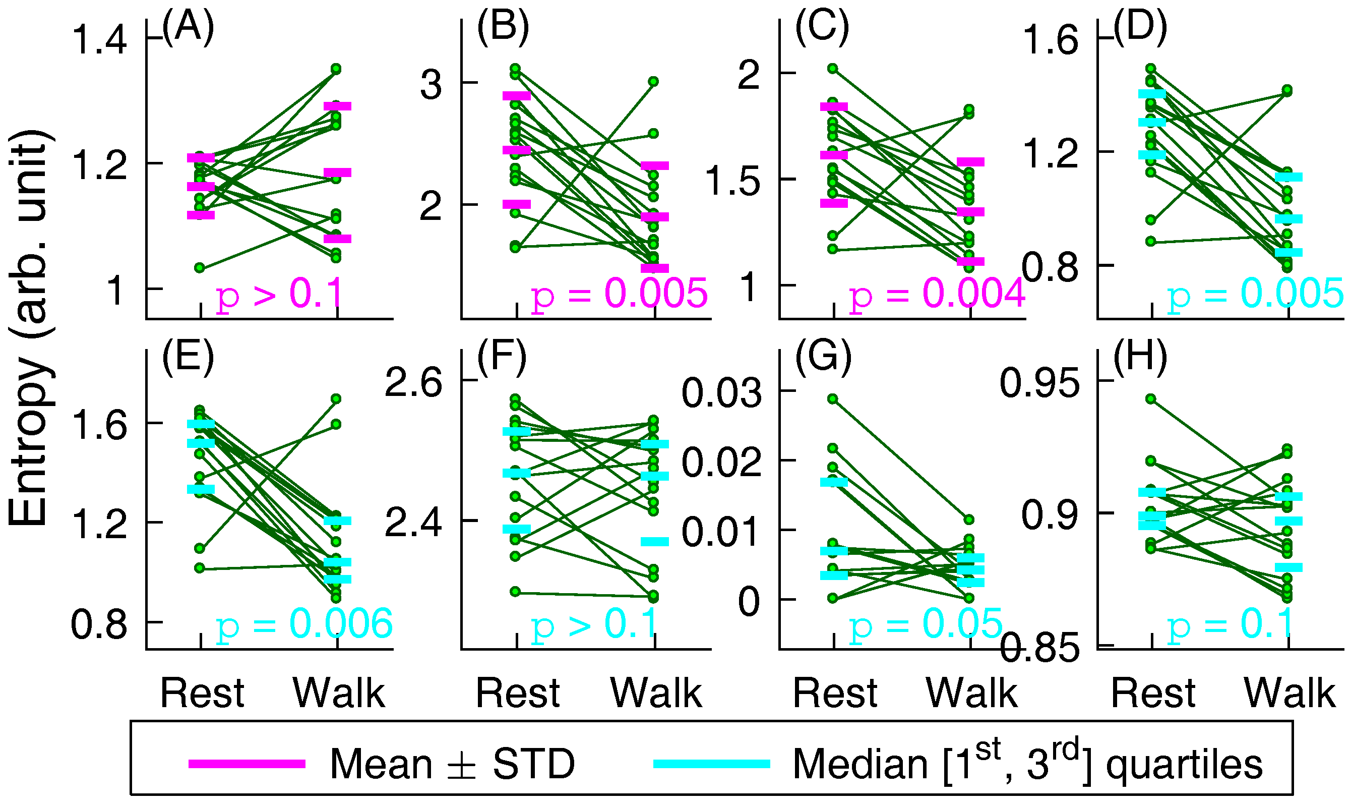
An average of 375 (SD: 46; min: 307; max: 485) RR intervals were obtained from the 16 participants during the Rest protocol. During the Walk protocol, the average length of HRV was 576 (SD: 49; min: 500; max: 699; p < 0.0001 vs. Rest). The Shapiro-Wilk $W$ tests suggested normality for ApEn, cApEn, and SampEn (all $p>0.2$) while it refuted the normal distribution hypothesis for the rest measures (all $p<0.05$) except DistEn, for which $p=0.07$. We here still considered DistEn non-normally distributed partly because the distribution, as visually checked, was less likely to follow a normal distribution and partly because of the relatively small sample size. Therefore, paired $t$-test was applied to examine the differences in ApEn, cApEn, and SampEn between Rest and Walk protocols, whereas for the rest five measures, Wilcoxon signed-rank test of each pair was applied.

Figure 1 shows the pair-wise changes of the eight entropy measures of HRV time-series before detrending between Rest and Walk conditions, with the corresponding mean (or median if non-normally distributed) and SD (or the 1st and 3rd quartiles) specified by short bars. Since eight tests were performed, here a $p$ value of $\le 0.006$ ($0.05/8\approx 0.006$) was considered statistically significant using the Bonferroni criterion. The results show no significant changes between the Walk and Rest conditions in ApEn ($p=0.1$), cApEn ($p>0.1$), and SampEn ($p>0.1$) as suggested by the paired $t$-test, and no significant changes in FuzzyEn-g and FuzzyEn-l (both $p=0.008$), either, as indicated by the Wilcoxon signed-rank test. By contrast, CE and DistEn reduce significantly under Walk condition as indicated by the Wilcoxon signed-rank test (all $p\le 0.006$). Large or even very large effect sizes are observed (i.e., $d=0.90$ for CE; $d=1.7$ for DistEn). PermEn however increases significantly under Walk condition ($p<0.0001$) with very large effect size ($d=1.9$).

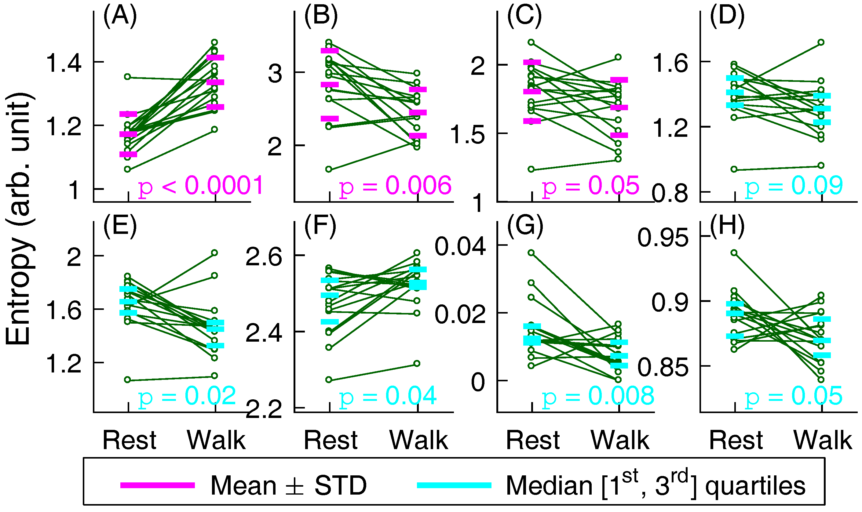
The results after linear detrending are shown in Figure 2. There is still no significant change in ApEn ($p>0.1$). Moreover, the observed changes in PermEn, CE, and DistEn become not significant (all $p>0.05$). However, the results show significantly reduced cApEn, SampEn, FuzzyEn-g, and FuzzyEn-l during Walk condition (all $p<0.006$) with large effect sizes (all $0.8<d<1$). Figure 3 shows the results after wavelet detrending. Surprisingly, ApEn shows a significant increase during Walk condition ($p<0.0001$; $d=1.9$). Similar to the result after linear detrending, cApEn decreases significantly ($p=0.006$; $d=0.8$). However, all the rest entropy measures do not indicate significant changes (all $p\ge 0.02$).

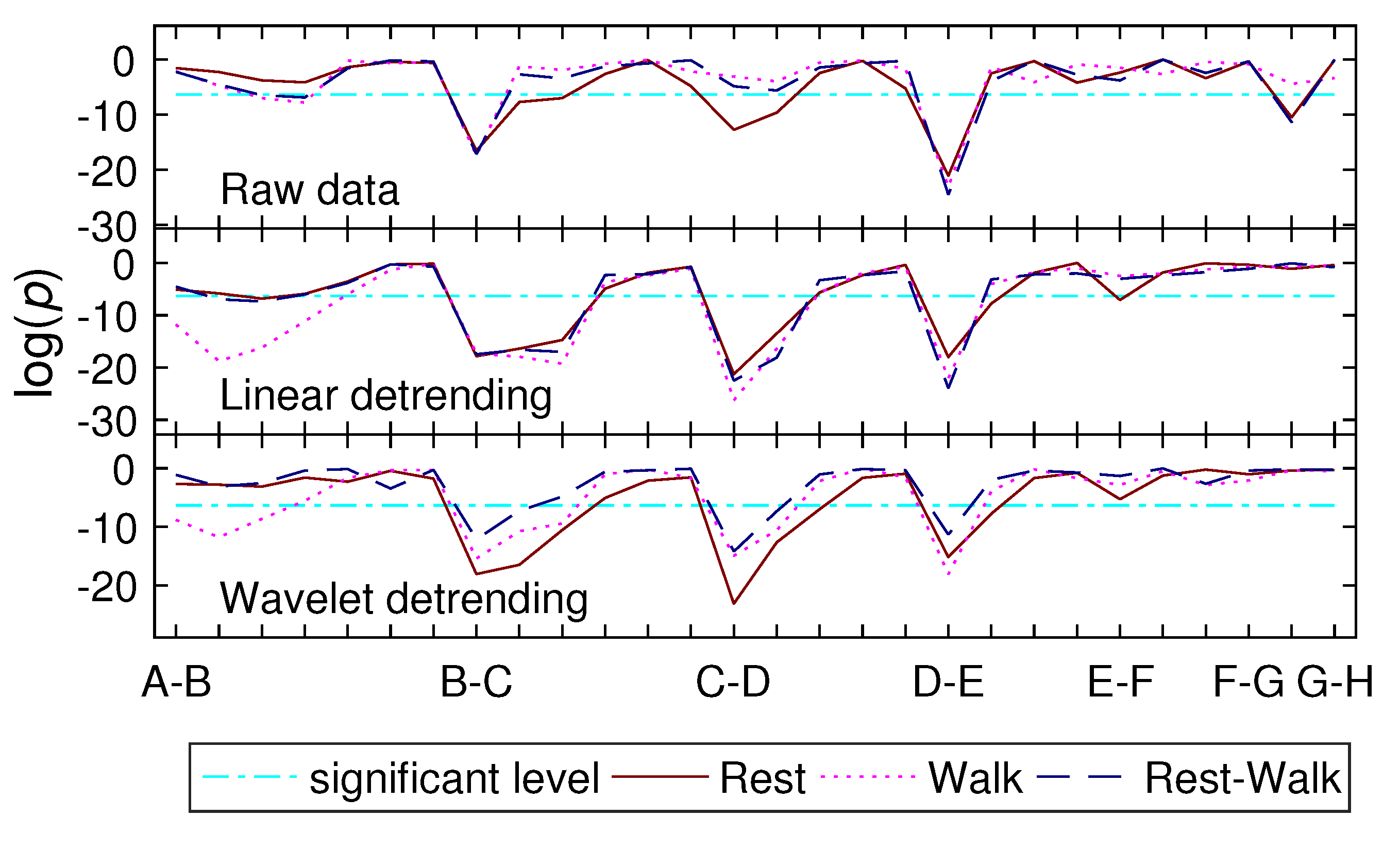
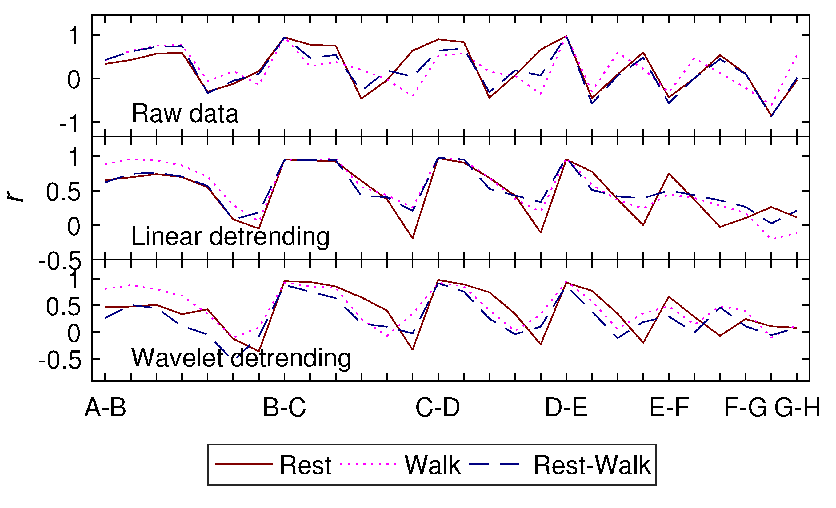
The bivariate Pearson correlation analysis results are showed in Figure 4 (which shows the test significance $p$) and Figure 5 (which shows the Pearson $r$). Results are summarized below.

1. For raw HRV time-series without detrending (upper panels in Figure 4 and Figure 5)

Under Rest condition, cApEn is positively correlated with SampEn, FuzzyEn-g, and FuzzyEn-l; SampEn is positively correlated with FuzzyEn-g and FuzzyEn-l; FuzzyEn-g is positively correlated with FuzzyEn-l; PermEn is negatively correlated with DistEn; no significant correlations are observed between all other pairs.

Under Walk condition, ApEn is positively correlated with FuzzyEn-g and FuzzyEn-l; c-ApEn is positively correlated with SampEn; FuzzyEn-g is positively correlated with FuzzyEn-l; no significant correlations are observed between the rest pairs.

Since many correlation results change during walking, those entropy measures are less likely to reproduce each other. Their responses to change of conditions may also be different. In order to illustrate this assumption, the bivariate correlation analysis between the pair-wise changes of entropy measures from Rest to Walk was also performed and the results are superimposed on those for Rest and Walk conditions in Figure 4 and Figure 5. The results are similar to those under Walk condition, except that the difference of PermEn is negatively correlated with the difference of DistEn, which is the same to that under Rest condition.

2. For HRV time-series after linear detrending (middle panels in Figure 4 and Figure 5)

The results are similar to those for raw HRV data, except that the negative correlation between PermEn and DistEn disappears. The results for Rest-Walk differences are the same to those for Rest condition. However, under Walk condition, in addition to those significant pairs for Rest condition, ApEn also shows positive correlations with cApEn, SampEn, FuzzyEn-g, and FuzzyEn-l.

3. For HRV time-series after wavelet detrending (lower panels in Figure 4 and Figure 5)

The results are exactly the same to those for HRV data after linear detrending except some changes in $p$ and $r$ values.

4. Discussion

Based on eight well-established entropy measures, we studied the within-subject changes of HRV during walking with a regular speed of 5 km/h on a treadmill (the Walk protocol) compared to those in a resting seated position (the Rest protocol). We also explored the potential effects of nonstationary linear, or very low-frequency trend. Our main findings are summarized in

Table 2. Summary of findings.

HRV vs. Measures 1	A	B	C	D	E	F	G	H
Raw	- 2	-	-	-	-	${\uparrow }^{ 3}$	${\downarrow }^{ 4}$	$\downarrow$
After linear detrending	-	$\downarrow$	$\downarrow$	$\downarrow$	$\downarrow$	-	-	-
After wavelet detrending	$\uparrow$	$\downarrow$	-	-	-	-	-	-

¹ A: ApEn; B: cApEn; C: SampEn; D: FuzzyEn-g; E: FuzzyEn-l; F: PermEn; G: CE; H: DistEn; ² No statistical significance; ³ Statistically significant increase; ⁴ Statistically significant decrease.

.

Even though the significant observations in PermEn, CE, and DistEn disappeared after linear or wavelet detrending, the changing directions were unchanged (i.e., walking leads to increased PermEn while decreased CE and DistEn, see Figure 1, Figure 2 and Figure 3). The insignificant results might be due to lack of power because only 16 subjects were enrolled. This is one of our study limitations. However, the within-subject design we applied may help improve the power. We are planning to enroll more participants and use a field protocol to further investigate the effects of daily activity.

Those findings suggest that the information that PermEn, CE, and DistEn capture may easily be “masked” by nonstationary trend which makes them less able to probe the changes in dynamics that are beyond the trend. Besides, PermEn is considered to be highly sensitive to noise [37] while few knowledge is known regarding the robustness of CE and DistEn against noise. The relative contribution of noise is supposed to be augmented after trend removal (which reduces signal power and thus reduces the signal-to-noise ratio). Noise in RR intervals may come from the tiny deviations between the detected and real R peaks (random noise) because of fixed rate sampling or spikes because of false positive or false negative detection, or ectopic beats. As we have mentioned in Method section, we conducted a thorough visual inspection regarding detection error and confirmed that no ectopic beats occurred. So only random noise may be considered as one of the factors that may affect our results. Besides, we note that the sampling frequency of the device we used is relatively low (200 Hz) which is considered to be another study limitation. The low sampling rate may lead to increased noise power that exacerbates the adverse effects on entropy measures.

SampEn, FuzzyEn-g, and FuzzyEn-l showed significant decrease during walking after linear detrending while the results became not significant again after wavelet detrending. Though seemingly erratic, the results are actually consistent to some extent as all the changing directions remain the same (Figure 1, Figure 2 and Figure 3). These findings imply that a linear detrend may be considered prior to performing the SampEn, FuzzyEn-g, and FuzzyEn-l analyses. The cApEn decreased significantly during walking after both linear and wavelet detrending (Figure 2 and Figure 3), which also suggests performing a detrend before using this method, irrelative to detrend methods. The ApEn only showed a significant difference between resting and walking conditions after wavelet detrending, suggesting ApEn highly sensitive to nonstationary trend. As a result, removal of nonstationary, very low-frequency trend should be performed before ApEn analysis.

However, there is little knowledge on whether or not the very low frequency trend contains useful physiological information. Those suggestions, as described above, are thus purely observation-based. Comprehensive studies on how nonstationary trend affects entropy analysis and further physiological investigations on the meaning of HRV trend are warranted. Anyway, the interpretation does differ from each other if different strategies are applied. For example, the insignificant ApEn observation on raw HRV and HRV after linear detrending might be due to the biasness of the ApEn algorithm as it includes self-matches [24], but ApEn became capable after wavelet detrending which seems to refute the possibility of biasness. However, considering the methodology, the number of similar vectors indeed increases after removing the trend component which thus reduces the weight of self-matches.

One interesting finding is that the changing direction of ApEn was opposite of cApEn and the other SampEn-based measures (i.e., SampEn, FuzzyEn-g, and FuzzyEn-l). Methodologically, both ApEn and SampEn assess the creation of information, or the unpredictability, in a time series [24]. The cApEn is basically a modified version of ApEn such that it is supposed to capture similar properties [31]. So does FuzzyEn which is actually a modified version of SampEn based on fuzzy logic [25,32]. However, the results come out to be that cApEn performs more similarly as SampEn does, instead of ApEn itself. This is also supported by the correlation analysis which showed that cApEn was always highly correlated to SampEn (i.e., $r$ value is very close to 1). The correction algorithm in cApEn may actually be equivalent to what SampEn applies. ApEn thus captures certain property hidden in the fluctuations that is different from SampEn-based measures.

The other interesting finding is that PermEn also shows different changing direction as compared to SampEn-based measures, CE, and DistEn. PermEn estimates the diversity of fluctuation patterns which may reflect the randomness [26]. CE functions like SampEn except that it estimates the average amount of information based on encoded time-series [27]. DistEn assesses actually the diversity of vectors in the state-space representation of a time-series [28]. Based on these methodological differences, the properties captured by different entropy measures may actually be intrinsically different or be different aspects of the complexity of HRV.

Overall, several other reasons may also contribute to the observed discrepancies across these entropy measures:

• All calculations were based on fixed input parameters which may not work well all the time. In other words, some results might not be completely true because improper parameters were applied. In the current study, we did not repeat our analyses using different combinations of parameters partly because that it would make things rather cumbersome for real application. Furthermore, there is no solid way to find out a proper choice for each individual case even though different combinations are able to be traversed. Previous studies have explored how to define parameters but the proposed approaches are mostly achieved retrospectively by maximizing the pre-hypothesized group differences [38,39,40]. However, it is not necessarily be always true that those hypothesized group differences exist.
• From the perspective of the underlying physiological mechanisms, it is still yet to be determined which branch in the ANS (i.e., sympathetic or vagal nerves) actually becomes dominant during walking at such a relatively lower but regular (for typical populations) speed. Some studies indicated that vagal withdrawal is the dominant mechanisms during lower intensity, dynamic exercise while others also points to a sympathetic HR modulation even at the onset of exercise [13,15]. Studies also suggested that the relative role of the two drives may depend on the exercise intensity [41]. It has been hypothesized that the withdrawal of parasympathetic (vagal) modulation might already be obvious during low intensity exercise, whereas the sympathetic increase may present at higher intensity exercises [17]. In addition, it is also controversial whether sympathetic drive to the heart or vagal withdrawal is the main contributor of HR complexity [21,31,42,43], let alone each specific complexity measure.

In term of sensitivity to the stimuli of regular walking, different measures actually indicate different sensitivity regarding different strategies applied for detrending. When raw HRV without detrending is used, PermEn and DistEn suggest the best sensitivity. The cApEn, SampEn, FuzzyEn-g, and FuzzyEn-l show comparable sensitivity for HRV after linear detrending. When wavelet detrending is applied, ApEn, however, suggests the best performance.

CE was not correlated with any other entropies under both Rest and Walk conditions, suggesting that it may capture a unique HRV nonlinear property. However, as shown in Figure 1G, CE under Rest condition distributed more dispersedly even though an overall significant reduction was displayed. Besides, many CE results actually researched the theoretical lower limit and this floor effect might introduce some bias in the estimation of effect size. This lack of robustness may thus deserve further elucidations. By contrast, DistEn showed correlation with SampEn and PermEn under Rest condition while under Walk condition no significant correlations were shown. Besides, no significant correlations between DistEn and others were observed for HRV after linear or wavelet detrending during both conditions. These results also render DistEn a unique role in analyzing HRV.

As a brief conclusion, when applying entropy analyses to short-term HRV data, we suggest: (1) using PermEn or DistEn on raw short-term HRV data; (2) performing linear detrend before applying SampEn-based measures; and (3) removing the very-low frequency trend before ApEn analysis. In order to make results comparable and to help better interpret different observations, whether or not detrend is performed as well as what detrending method is applied should be clearly specified.

With the rapid advances of technology and reduced cost, the use of wearable devices that are able to monitor heart rate continuously will likely become rather commonplace. Our current study shows that regular walking may acutely affect the commonly applied HRV entropies. The effect of daily activities should therefore be taken into consideration when interpreting results from long-time ambulatory recordings. Device developers may consider including event reporters in those devices for users to track their activities throughout the day, which can be a useful reference for data analyses. In our future studies, field protocols will be designed to examine the effects of real daily activities.

References

- Hayano, J.; Sakakibara, Y.; Yamada, A.; Yamada, M.; Mukai, S.; Fujinami, T.; Yokoyama, K.; Watanabe, Y.; Takata, K. Accuracy of assessment of cardiac vagal tone by heart rate variability in normal subjects. Am. J. Cardiol. 1991, 67, 199–204. [Google Scholar] [CrossRef]
- Ziegler, D.; Voss, A.; Rathmann, W.; Strom, A.; Perz, S.; Roden, M.; Peters, A.; Meisinger, C.; Group, K.S. Increased prevalence of cardiac autonomic dysfunction at different degrees of glucose intolerance in the general population: The kora s4 survey. Diabetologia 2015, 58, 1118–1128. [Google Scholar] [CrossRef] [PubMed]
- Felber Dietrich, D.; Schindler, C.; Schwartz, J.; Barthelemy, J.C.; Tschopp, J.M.; Roche, F.; von Eckardstein, A.; Brandli, O.; Leuenberger, P.; Gold, D.R.; et al. Heart rate variability in an ageing population and its association with lifestyle and cardiovascular risk factors: Results of the sapaldia study. Europace 2006, 8, 521–529. [Google Scholar] [CrossRef] [PubMed]
- Tsuji, H.; Venditti, F.J., Jr.; Manders, E.S.; Evans, J.C.; Larson, M.G.; Feldman, C.L.; Levy, D. Reduced heart rate variability and mortality risk in an elderly cohort. The framingham heart study. Circulation 1994, 90, 878–883. [Google Scholar] [CrossRef] [PubMed]
- Drawz, P.; Babineau, D.; Brecklin, C.; He, J.; Kallem, R.; Soliman, E.; Xie, D.; Appleby, D.; Anderson, A.; Rahrnan, M.; et al. Heart rate variability is a predictor of mortality in chronic kidney disease: A report from the cric study. Am. J. Nephrol. 2013, 38, 517–528. [Google Scholar] [CrossRef] [PubMed]
- Ziegler, D.; Zentai, C.P.; Perz, S.; Rathmann, W.; Haastert, B.; Döring, A.; Meisinger, C.; Group, K.S. Prediction of mortality using measures of cardiac autonomic dysfunction in the diabetic and nondiabetic population: The monica/kora augsburg cohort study. Diabetes Care 2008, 31, 556–561. [Google Scholar] [CrossRef] [PubMed]
- Dekker, J.M.; Crow, R.S.; Folsom, A.R.; Hannan, P.J.; Liao, D.; Swenne, C.A.; Schouten, E.G. Low heart rate variability in a 2-minute rhythm strip predicts risk of coronary heart disease and mortality from several causes: The aric study. Atherosclerosis risk in communities. Circulation 2000, 102, 1239–1244. [Google Scholar] [CrossRef] [PubMed]
- Liao, D.; Cai, J.; Rosamond, W.D.; Barnes, R.W.; Hutchinson, R.G.; Whitsel, E.A.; Rautaharju, P.; Heiss, G. Cardiac autonomic function and incident coronary heart disease: A population-based case-cohort study. The aric study. Atherosclerosis risk in communities study. Am. J. Epidemiol. 1997, 145, 696–706. [Google Scholar] [CrossRef] [PubMed]
- Akintola, A.A.; van de Pol, V.; Bimmel, D.; Maan, A.C.; van Heemst, D. Comparative analysis of the equivital eq02 lifemonitor with holter ambulatory ecg device for continuous measurement of ecg, heart rate, and heart rate variability: A validation study for precision and accuracy. Front. Physiol. 2016, 7, 391. [Google Scholar] [CrossRef] [PubMed]
- Kristiansen, J.; Korshoj, M.; Skotte, J.H.; Jespersen, T.; Sogaard, K.; Mortensen, O.S.; Holtermann, A. Comparison of two systems for long-term heart rate variability monitoring in free-living conditions—A pilot study. Biomed. Eng. Online 2011, 10, 27. [Google Scholar] [CrossRef] [PubMed] [Green Version]
- Morris, C.J.; Purvis, T.E.; Hu, K.; Scheer, F.A. Circadian misalignment increases cardiovascular disease risk factors in humans. Proc. Natl. Acad. Sci. USA 2016, 113, E1402–E1411. [Google Scholar] [CrossRef] [PubMed]
- Taylor, K.A.; Wiles, J.D.; Coleman, D.D.; Sharma, R.; O’Driscoll, J.M. Continuous cardiac autonomic and haemodynamic responses to isometric exercise. Med. Sci. Sports Exerc. 2017. [Google Scholar] [CrossRef] [PubMed]
- White, D.W.; Raven, P.B. Autonomic neural control of heart rate during dynamic exercise: Revisited. J. Physiol. 2014, 592, 2491–2500. [Google Scholar] [CrossRef] [PubMed]
- Weippert, M.; Behrens, M.; Rieger, A.; Behrens, K. Sample entropy and traditional measures of heart rate dynamics reveal different modes of cardiovascular control during low intensity exercise. Entropy 2014, 16, 5698–5711. [Google Scholar] [CrossRef]
- Fisher, J.P. Autonomic control of the heart during exercise in humans: Role of skeletal muscle afferents. Exp. Physiol. 2014, 99, 300–305. [Google Scholar] [CrossRef] [PubMed]
- Goya-Esteban, R.; Barquero-Perez, O.; Sarabia-Cachadina, E.; de la Cruz-Torres, B.; Naranjo-Orellana, J.; Rojo-Alvarez, J.; Murray, A. Heart rate variability non linear dynamics in intense exercise. Comput. Cardiol. 2012, 39, 177–180. [Google Scholar]
- Boettger, S.; Puta, C.; Yeragani, V.K.; Donath, L.; Muller, H.J.; Gabriel, H.H.; Bar, K.J. Heart rate variability, qt variability, and electrodermal activity during exercise. Med. Sci. Sports Exerc. 2010, 42, 443–448. [Google Scholar] [CrossRef] [PubMed]
- Leicht, A.S.; Sinclair, W.H.; Spinks, W.L. Effect of exercise mode on heart rate variability during steady state exercise. Eur. J. Appl. Physiol. 2008, 102, 195–204. [Google Scholar] [CrossRef] [PubMed]
- Princi, T.; Accardo, A.; Peterec, D. Linear and non-linear parameters of heart rate variability during static and dynamic exercise in a high-performance dinghy sailor. Biomed. Sci. Instrum. 2004, 40, 311–316. [Google Scholar] [PubMed]
- Cottin, F.; Durbin, F.; Papelier, Y. Heart rate variability during cycloergometric exercise or judo wrestling eliciting the same heart rate level. Eur. J. Appl. Physiol. 2004, 91, 177–184. [Google Scholar] [CrossRef] [PubMed]
- Tulppo, M.; Makikallio, T.; Takala, T.; Seppanen, T.; Huikuri, H. Quantitative beat-to-beat analysis of heart rate dynamics during exercise. Am. J. Physiol. Heart Circ. Physiol. 1996, 271, H244–H252. [Google Scholar]
- Sugihara, G.; Allan, W.; Sobel, D.; Allan, K.D. Nonlinear control of heart rate variability in human infants. Proc. Natl. Acad. Sci. USA 1996, 93, 2608–2613. [Google Scholar] [CrossRef] [PubMed]
- Pincus, S.M. Approximate entropy as a measure of system complexity. Proc. Natl. Acad. Sci. USA 1991, 88, 2297–2301. [Google Scholar] [CrossRef] [PubMed]
- Richman, J.S.; Moorman, J.R. Physiological time-series analysis using approximate entropy and sample entropy. Am. J. Physiol. Heart Circ. Physiol. 2000, 278, H2039–H2049. [Google Scholar] [PubMed]
- Chen, W.; Zhuang, J.; Yu, W.; Wang, Z. Measuring complexity using fuzzyen, apen, and sampen. Med. Eng. Phys. 2009, 31, 61–68. [Google Scholar] [CrossRef] [PubMed]
- Bandt, C.; Pompe, B. Permutation entropy: A natural complexity measure for time series. Phys. Rev. Lett. 2002, 88, 174102. [Google Scholar] [CrossRef] [PubMed]
- Porta, A.; Baselli, G.; Liberati, D.; Montano, N.; Cogliati, C.; Gnecchi-Ruscone, T.; Malliani, A.; Cerutti, S. Measuring regularity by means of a corrected conditional entropy in sympathetic outflow. Biol. Cybern. 1998, 78, 71–78. [Google Scholar] [CrossRef] [PubMed]
- Li, P.; Liu, C.; Li, K.; Zheng, D.; Liu, C.; Hou, Y. Assessing the complexity of short-term heartbeat interval series by distribution entropy. Med. Biol. Eng. Comput. 2015, 53, 77–87. [Google Scholar] [CrossRef] [PubMed]
- Li, P.; Karmakar, C.; Yan, C.; Palaniswami, M.; Liu, C. Classification of five-second epileptic eeg recordings using distribution entropy and sample entropy. Front. Physiol. 2016, 7, 136. [Google Scholar] [CrossRef] [PubMed]
- Li, P.; Liu, C.; Zhang, M.; Che, W.; Li, J. A real-time qrs complex detection method. Acta Biophys. Sin. 2011, 27, 222–230. [Google Scholar] [CrossRef]
- Porta, A.; Gnecchi-Ruscone, T.; Tobaldini, E.; Guzzetti, S.; Furlan, R.; Montano, N. Progressive decrease of heart period variability entropy-based complexity during graded head-up tilt. J. Appl. Physiol. (1985) 2007, 103, 1143–1149. [Google Scholar] [CrossRef] [PubMed]
- Liu, C.; Li, K.; Zhao, L.; Liu, F.; Zheng, D.; Liu, C.; Liu, S. Analysis of heart rate variability using fuzzy measure entropy. Comput. Biol. Med. 2013, 43, 100–108. [Google Scholar] [CrossRef] [PubMed]
- Li, P.; Li, K.; Liu, C.; Zheng, D.; Li, Z.-M.; Liu, C. Detection of coupling in short physiological series by a joint distribution entropy method. IEEE Trans. Biomed. Eng. 2016, 63, 2231–2242. [Google Scholar] [CrossRef] [PubMed]
- Makowiec, D.; Kaczkowska, A.; Wejer, D.; Żarczyńska-Buchowiecka, M.; Struzik, Z. Entropic measures of complexity of short-term dynamics of nocturnal heartbeats in an aging population. Entropy 2015, 17, 1253–1272. [Google Scholar] [CrossRef]
- Karmakar, C.; Udhayakumar, R.K.; Li, P.; Venkatesh, S.; Palaniswami, M. Stability, consistency and performance of distribution entropy in analysing short length heart rate variability (hrv) signal. Front. Physiol. 2017, 8, 720. [Google Scholar] [CrossRef] [PubMed]
- Sawilowsky, S.S. New effect size rules of thumb. J. Mod. Appl. Stat. Methods 2009, 8, 597–599. [Google Scholar] [CrossRef]
- Porta, A.; Bari, V.; Marchi, A.; De Maria, B.; Castiglioni, P.; di Rienzo, M.; Guzzetti, S.; Cividjian, A.; Quintin, L. Limits of permutation-based entropies in assessing complexity of short heart period variability. Physiol. Meas. 2015, 36, 755–765. [Google Scholar] [CrossRef] [PubMed]
- Liu, C.; Liu, C.; Shao, P.; Li, L.; Sun, X.; Wang, X.; Liu, F. Comparison of different threshold values r for approximate entropy: Application to investigate the heart rate variability between heart failure and healthy control groups. Physiol. Meas. 2011, 32, 167–180. [Google Scholar] [CrossRef] [PubMed]
- Lu, S.; Chen, X.; Kanters, J.K.; Solomon, I.C.; Chon, K.H. Automatic selection of the threshold value r for approximate entropy. IEEE Trans. Biomed. Eng. 2008, 55, 1966–1972. [Google Scholar] [PubMed]
- Li, P.; Liu, C.; Wang, X.; Li, L.; Yang, L.; Chen, Y.; Liu, C. Testing pattern synchronization in coupled systems through different entropy-based measures. Med. Biol. Eng. Comput. 2013, 51, 581–591. [Google Scholar] [CrossRef] [PubMed]
- Aubert, A.E.; Seps, B.; Beckers, F. Heart rate variability in athletes. Sports Med. 2003, 33, 889–919. [Google Scholar] [CrossRef] [PubMed]
- Porta, A.; Castiglioni, P.; Bari, V.; Bassani, T.; Marchi, A.; Cividjian, A.; Quintin, L.; Di Rienzo, M. K-nearest-neighbor conditional entropy approach for the assessment of the short-term complexity of cardiovascular control. Physiol. Meas. 2013, 34, 17–33. [Google Scholar] [CrossRef] [PubMed]
- Porta, A.; Guzzetti, S.; Furlan, R.; Gnecchi-Ruscone, T.; Montano, N.; Malliani, A. Complexity and nonlinearity in short-term heart period variability: Comparison of methods based on local nonlinear prediction. IEEE Trans. Biomed. Eng. 2007, 54, 94–106. [Google Scholar] [CrossRef] [PubMed]
Figure 1.
The entropies of raw short-term heartbeat interval series. In order to show the changes, results from the same participants were connected by lines.
(A) ApEn; (B) cApEn; (C) SampEn; (D) FuzzyEn-g; (E) FuzzyEn-l; (F) PermEn; (G) CE; (H) DistEn.
Figure 2.
The entropies of short-term heartbeat interval series after linear detrending. In order to show the changes, results from the same participants were connected by lines. (A) ApEn; (B) cApEn; (C) SampEn; (D) FuzzyEn-g; (E) FuzzyEn-l; (F) PermEn; (G) CE; (H) DistEn.
Figure 3.
The entropies of short-term heartbeat interval series after wavelet detrending. In order to show the changes, results from the same participants were connected by lines. (A) ApEn; (B) cApEn; (C) SampEn; (D) FuzzyEn-g; (E) FuzzyEn-l; (F) PermEn; (G) CE; (H) DistEn.
Figure 4.
Bivariate correlation analysis results. The abscissa shows between which two entropy measures the correlation analysis was performed. The codes A to H mean ApEn, cApEn, SampEn, FuzzyEn-g, FuzzyEn-l, PermEn, CE, and DistEn, respectively. The label ‘A-B’ thus indicates the correlation between ApEn and cApEn, and so do the rest labels. The values are shown in logarithmic scale in the ordinate, such that a significant test result is obtained if the corresponding value is less than the significant level, which is after Bonferroni correction.
Figure 5.
Bivariate correlation analysis results. Results are shown in the same way as has applied in Figure 4, except that the ordinate is showing the Pearson .