Fire and the Distribution and Uncertainty of Carbon Sequestered as Aboveground Tree Biomass in Yosemite and Sequoia & Kings Canyon National Parks

Abstract

Fire is one of the principal agents changing forest carbon stocks and landscape level distributions of carbon, but few studies have addressed how accurate carbon accounting of fire-killed trees is or can be. We used a large number of forested plots (1646), detailed selection of species-specific and location-specific allometric equations, vegetation type maps with high levels of accuracy, and Monte Carlo simulation to model the amount and uncertainty of aboveground tree carbon present in tree species (hereafter, carbon) within Yosemite and Sequoia & Kings Canyon National Parks. We estimated aboveground carbon in trees within Yosemite National Park to be 25 Tg of carbon (C) (confidence interval (CI): 23–27 Tg C), and in Sequoia & Kings Canyon National Park to be 20 Tg C (CI: 18–21 Tg C). Low-severity and moderate-severity fire had little or no effect on the amount of carbon sequestered in trees at the landscape scale, and high-severity fire did not immediately consume much carbon. Although many of our data inputs were more accurate than those used in similar studies in other locations, the total uncertainty of carbon estimates was still greater than ±10%, mostly due to potential uncertainties in landscape-scale vegetation type mismatches and trees larger than the ranges of existing allometric equations. If carbon inventories are to be meaningfully used in policy, there is an urgent need for more accurate landscape classification methods, improvement in allometric equations for tree species, and better understanding of the uncertainties inherent in existing carbon accounting methods.

1. Introduction

The distribution and abundance of aboveground carbon sequestered in trees and snags (hereafter, carbon) in western North America are of crucial importance to land management issues related to fire [1] and climate [2]. Total fuel loading, of which the principal component is the aboveground portion of trees and snags, is increasingly important to the level of fire risk in cities, suburbs, and exurban areas around the world [3]. In the Sierra Nevada, the period of fire suppression in the 1900s greatly changed the structure and composition of forests [4], posing challenges for restoration. The amount of carbon reflects the history of disturbance and gradients of productivity [5,6]. However, detailed estimates of carbon have many sources of variation that are difficult to quantify for any particular landscape (e.g., [7,8]). The heterogeneity of vegetation types on the landscape, the structural variation within types, and the belowground carbon pools lead to significant challenges in characterizing and modeling carbon stocks at landscape or across landscape scales and propagating the various sources of error in the final estimate (e.g., [9,10]).

Whereas most studies have focused on aboveground tree carbon pools, very few have attempted to characterize carbon at or below the soil surface. These latter carbon pools include shrubs, woody debris, litter, soil organic and mineral horizons, and live and dead roots [11,12,13,14]. These sources contain significant amounts of carbon, which can represent over half of the total carbon in boreal forests and somewhat less than half in tropical forests [15]. The temperate forests of the Sierra Nevada are thought to fall somewhere in between, with the amount of non-tree carbon varying with tree canopy cover [16]. Due to the variability of carbon stocks at or below the soil surface, and the limited number of studies that describe them, we focus instead on carbon in the aboveground components of trees, which are thought to constitute at least half of the total carbon in the forests of the Sierra Nevada.

Current techniques for estimating aboveground carbon rely on the scaling of tree allometries to the landscape level. Tree inventories are converted to areal estimates of carbon using allometric equations for a given vegetation type, and landscape level values are calculated based on the distribution of those vegetation types. Landscape vegetation classes are often developed from relatively coarse Landsat-derived maps. Although this approach allows for formulaic extrapolation to the landscape or ecoregion, most such schemes (e.g., NASA-CASA [17,18]) do not propagate the associated errors. We identified five potentially large sources of error associated with this approach to estimating carbon across large landscapes and grouped them into two broad categories—allometry and landscape classification.

1.1. Potential Errors Related to Allometry

(1)

Tree allometric equations themselves—tree level allometric equations are usually derived from a small number of trees (typically <25, but often <10 [19]), and the effects of model selection can greatly influence results [20]. The allometric equations often have considerable standard errors—usually 10% to 30% of the range of tree diameters used to develop them.

(2)

Site-specific tree morphology—trees sampled for allometric equations usually represent only one portion of the species range. When the equations are applied elsewhere, differences in site productivity, disturbance history, and climate could yield errors due to different morphologies between the sampled and target populations.

(3)

Lack of large-diameter tree representation—few allometric equations are derived from samples of large trees, with very few tree dissections having occurred for trees >100 cm diameter at breast height (dbh). Therefore, the biomass of large-diameter trees must be estimated from those few proxy species that have been sampled at large diameters. The problem of accurately calculating the biomass of large-diameter trees is magnified by their more complex and variable crown architecture [21,22]. Importantly, large-diameter trees contain a large proportion of the biomass of Sierra Nevada forests [11]. Therefore, in areas where large-diameter trees exist, particularly where individuals reach maximum sizes much greater than any previously dissected, biomass estimates could potentially have large uncertainties.

1.2. Potential Errors Related to Landscape Classification and Mapping

(4)

Landscape heterogeneity—landscape level estimates of carbon must be based on a sufficient number of plots to capture the range in vegetation conditions and their representation on the landscape [23]. Although the present study used a sufficient number of forest plots (1646), studies with too few plots to represent the landscape heterogeneity also may have errors related to the time since disturbance, a principal contributor to heterogeneity [24].

(5)

Vegetation type mismatch—when plot level data are scaled to the landscape, errors in vegetation cover assignment can yield errors in scaled biomass.

These sources of error make determination of an exact number for carbon sequestration problematic, and single number estimates may be problematic if applied to policy or management decisions. Rather, the likely range of values for carbon sequestration and an appreciation of the uncertainties may be more important [10]. We sought to make the best attainable calculation of carbon stocks for two National Parks in the Sierra Nevada, and through simulation, estimate the effect that errors in each of the five categories of uncertainties could have in an estimate of landscape carbon.

Yosemite and Sequoia & Kings Canyon National Parks represent two heterogeneous landscapes where carbon sequestration is a management priority but difficult to quantify. Although landscape-scale heterogeneity of forest structure in the Sierra Nevada, and its response to fire, is well established by remote sensing studies [25,26,27], we lack a crosswalk between forest structural metrics and carbon abundance. Developing a method for this translation has proved challenging in part because the heterogeneity of carbon across these landscapes arises from nearly every ecological process: the species present [28], the productivity gradient [6], the history and magnitude of fire and wind [29,30,31,32], fuels treatment and management [33], dispersal and post-disturbance forest development [34], and the effects of insects and pathogens. The ubiquity of these mechanisms of heterogeneity increases the difficulty of quantifying carbon stocks: morphological variation within species expands the error associated with allometric equations; adequate sample breadth among community types and disturbance histories is difficult to attain, and mapping inaccuracies are difficult to avoid. Here, we address the following objectives: (1) to generate landscape-scale estimates of aboveground carbon in woody stems as accurately as possible with current geographic and allometric data; (2) to quantify uncertainties associated with allometric equations, specifically those related to diameter measurement error, and mapping inaccuracies; and (3) to assess effects of low-, moderate-, and high-severity fire on carbon stocks.

2. Materials and Methods

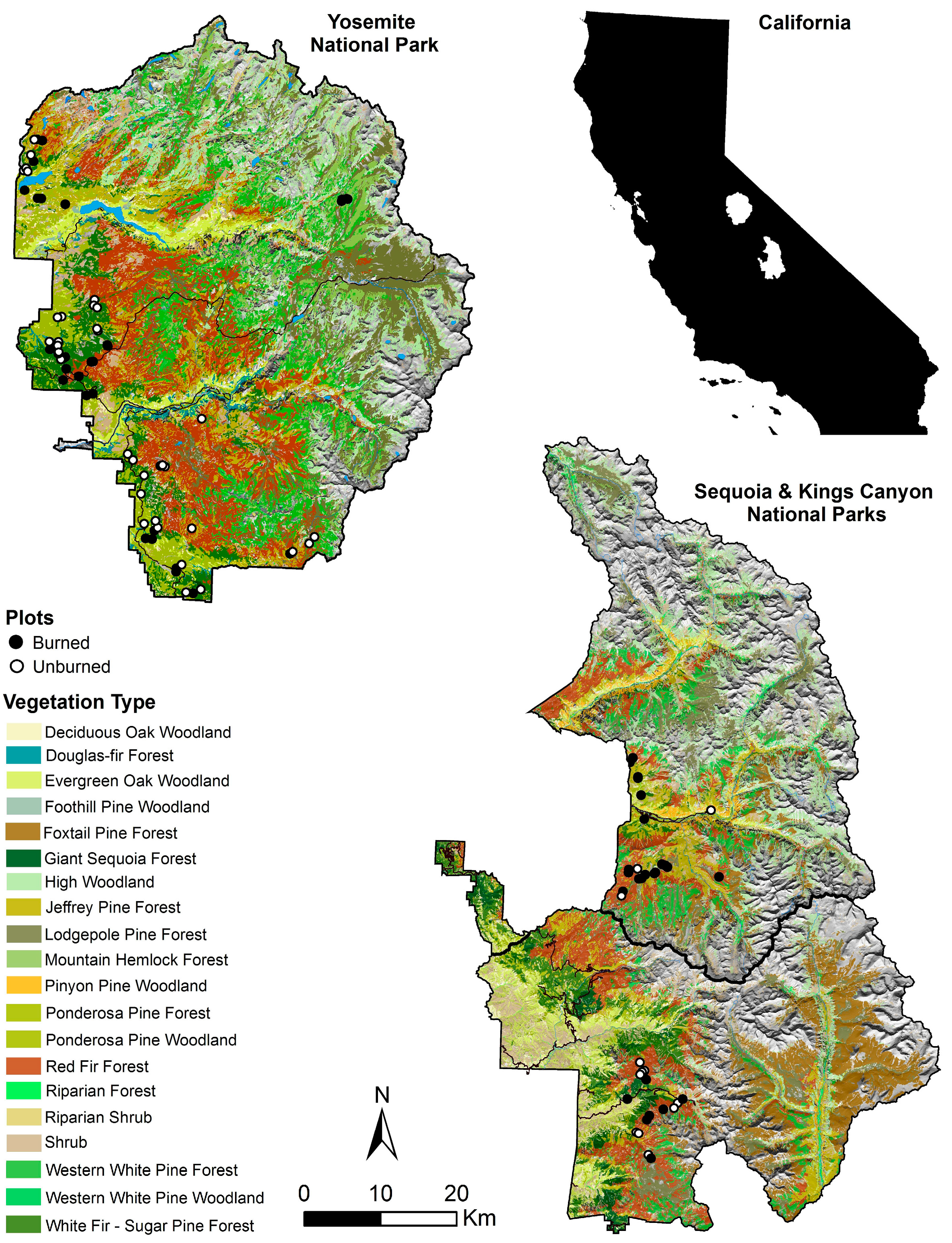
2.1. Study Area

Yosemite National Park (Yosemite) and Sequoia & Kings Canyon National Parks (Sequoia) are located in central to southern Sierra Nevada, California, USA (Figure 1). Yosemite extends over 3027 km² with elevations ranging from 648 m to 3997 m, and Sequoia extends over 3504 km², with elevations ranging from 520 m to 4418 m. Both Yosemite and Sequoia are primarily vegetated with coniferous forests and woodlands (57%), with lesser portions of deciduous forests and woodlands (6%) and chaparral (8%) [35,36]. Both parks contain considerable unvegetated areas at high elevations or on rocky outcrops (29%).

The fire regime is mixed, with lower elevations generally having experienced frequent, low-severity fire prior to the onset of fire suppression in the early 20th century [31]. Forest structure and fire effects are strongly influenced by topography and water balance, resulting in a patchy distribution of forest types [37]. The approximately 100-year period of fire suppression has increased tree density in many lower elevation areas of the parks [38,39,40].

2.2. Plot Data

To estimate carbon, we combined field data from plot-based vegetation studies in Yosemite and Sequoia. Data were collected for different research objectives (carbon tabulation, fire effects monitoring, fuel monitoring, natural resource inventories, and vegetation community surveys), but all contained similar tree information (

Table 1. Number of sampling plots located within each consolidated vegetation type in Yosemite and Sequoia & Kings Canyon National Parks.

Consolidated Forest Vegetation Type	Number of Plots
Deciduous Oak Forest and Woodland	88
Douglas-fir Forest	7
Evergreen Oak Forest and Woodland	110
Foothill Pine Woodland	11
Foxtail Pine Forest	58
Giant Sequoia Forest	42
High Woodland	89
Jeffrey Pine Forest	111
Lodgepole Pine Forest	190
Mountain Hemlock Forest	38
Pinyon Pine Woodland	27
Ponderosa Pine Forest	123
Ponderosa Pine Woodland	13
Red Fir Forest	116
Riparian Forest	87
Riparian Shrub	23
Shrub	258
Western White Pine Forest	27
Western White Pine Woodland	4
White Fir—Sugar Pine Forest	224
Total	1646

). To supplement the pre-existing plot data, we established 115, 0.1 ha circular plots (Figure 1) in Yosemite (67 plots) and Sequoia (48 plots). These plots were stratified by five different vegetation cover types (Abies concolor-Pinus lambertiana [white fir-sugar pine], Abies magnifica [red fir], Pinus contorta [lodgepole pine], Pinus jeffreyi [Jeffrey pine], Pinus ponderosa [ponderosa pine]) and fire history (burned or unburned in recorded history). See [41,42] for detailed field methods.

2.3. Vegetation Mapping

We used vegetation maps compiled from aerial photography and plot data to estimate carbon stocks at the landscape level. High-resolution aerial photos (effective pixel size <0.5 m) were acquired for Yosemite in 1997 and in 2000 for Sequoia by low-flying aircraft, and vegetation was delineated by community type [42,43]. Teams experienced in photointerpretation and with extensive field experience in the Sierra Nevada delineated vegetation by community type and created vegetation maps where polygons corresponded to areas of consistent vegetation type and canopy cover.

The defined vegetation types in Yosemite and Sequoia [42] contain many similar community types with some containing few vegetation plots in our compiled dataset (or in some cases, none). Many similar vegetation types are differentiated based upon understory shrub and herbaceous species composition, whereas much of the carbon storage is driven by the composition and morphology of the dominant overstory species [44]. Fire return interval is also driven more by overstory vegetation and productivity than the precise vegetation community [31,45,46]. Thus, we consolidated many of the mapped types for the purpose of this carbon and fire analysis. For example, high elevation woodlands cover a considerable area of both parks, but have a generally low carbon density, very infrequent fire return interval, and characteristic tree morphology (short, conic boles). Based on the similarity of tree morphology (i.e., Sierra Juniper, whitebark pine, mountain hemlock), and therefore carbon content, and infrequent fire return interval, we used a single “carbon/fire type” for these vegetation communities. We consolidated the mapped vegetation types into 20 categories representing consistent carbon and fire behavior characteristics (Figure 1, Table 1).

2.4. Allometric Equations

We searched the existing literature (principally summarized in [19]) and allometric equation databases (e.g., BIOPAK [47]) and selected those equations that best represented the species and diameter classes present in Yosemite and Sequoia (full list in Appendix A). We consulted the original source manuscripts for the equations, and when selecting the most appropriate equation(s), we considered the geography of the original study, tree age range (where reported), tree diameter range, site productivity, site climate, and sample size. When available, we used species-specific or genus-specific equations from studies geographically closest to our study region (e.g., [48] for Abies). If a species-specific equation was not available, we chose an equation from a species with a similar growth form or used one of the generalized equations developed by Jenkins et al. [49]. However, in many cases, particularly the high elevation woodlands, the Jenkins et al. [49] generalized equations were not appropriate because of the small stature (relative to diameter) of high elevation individuals of Pinus and Tsuga. In these cases, we used proxy species with equations better matched to the lifeform of the target species in the Sierra Nevada (e.g., juniper [50]).

In many cases, the diameter ranges of trees used to develop an equation did not extend throughout the diameter range of trees in our dataset. Yosemite and Sequoia contain the largest (or nearly so) individuals of Pinus ponderosa, Pinus lambertiana, Abies concolor, Abies magnifica, and Sequoiadendron giganteum [51], and because destructive sampling is generally enjoined in the parks, allometric equations extending to those large diameters do not exist. For large-diameter trees, we created blended equations using species-specific equations over the diameter range of trees from which the equation was developed and equations from similar species and growth forms that covered the necessary extended diameter range. Some allometric equations (i.e., juniper) were based on basal diameter. For these trees, we converted between dbh and basal diameter using the taper equations of Demaerschaulk and Omule [52].

All equations were of the form ln(biomass) = a + b × ln(dbh), with ln representing the natural logarithm, biomass expressed in kg, and dbh given in cm. Each equation included the standard error of the estimate (SEE), which is the standard deviation of the normally-distributed error around the predicted biomass while expressed on a log scale, and can be used to calculate a bias correction factor when exponentiating the log-scaled biomass to an arithmetic value and for calculating the standard error of a tree’s estimated biomass. As the trees were principally temperate coniferous species, tree carbon mass was assumed to be 50% of biomass based on the proportion of carbon found in cellulose, hemicellulose, and lignin, but without regard for the various proportions of carbon present in species-specific complex organic compounds (e.g., polyphenols and extractives [53]). Although the proportion of carbon differs by species and tissue (wood, bark, and foliage), conifer species have a mean wood carbon value variously reported as 50.8% [53], or 47%–55% [54]. The 50% figure provides an acceptable average—generally, firs (Abies spp.) have carbon contents slightly less than 50%, pines (Pinus spp.) slightly greater than 50%, and the Sierra Nevada Cupressaceae around 52%. However, similar to the situation with allometric equations, very few carbon analyses have been done on the species prevalent in Yosemite and Sequoia.

We estimated tree carbon density (Mg·ha⁻¹ C) and total carbon (Tg C) for each forest type within each park. Our definition of trees included living trees and standing snags. In addition to the typical uncertainty in estimated statistical parameters arising from sampling a population, we also explored the influence of various other measurement errors on carbon estimates and their uncertainties. These measurement errors included repeatability in tree diameter measurements, uncertainties in allometric equation diameter–biomass relationships, and classification accuracies in vegetation maps. We developed a Monte Carlo simulation that repeatedly calculated carbon densities and total carbon while taking into account those uncertainties. For tree diameter, a normally-distributed error with mean 0 and standard deviation 0.027 (based on the RMSE of duplicated tree diameter measurements reported by Gonzalez et al. [55]) was added to each tree dbh measurement. Tree biomass was calculated using the assigned allometric equations. A normally-distributed error with mean 0 and standard deviation equal to the equation’s standard error of the estimate (SEE) was added (while biomass was on a log scale). Typically, when making a single prediction using a log-log equation, a bias correction is added to the value so that when it is exponentiated, it is closer to the arithmetic mean (the arithmetic values tend to be log-normally distributed and exponentiating the log value without bias correction will place the prediction closer to the distribution’s median [56]). However, during a Monte Carlo simulation, the distribution of multiple arithmetic predictions will realize the log-normal distribution, so a bias correction is not needed. Log-scaled tree biomass values were exponentiated, summed within a plot, and divided by the plot area to produce a carbon density value (Mg·ha⁻¹ C). A bootstrapped sample (a random sample with replacement equal in size to the original sample) of all plots was taken in order to incorporate uncertainty from statistical sampling. We then fit a linear regression model to predict carbon density (log + 1 transformed) using forest type, forest canopy cover class, and their interaction as explanatory variables. Forest canopy cover classes were taken from the forest type maps, where each mapped polygon had been assigned a canopy cover class during photo interpretation. Three forest types (Douglas-fir forest, foothill pine woodland, and western white pine woodland) did not have enough plots across a range of canopy covers, so their carbon estimates are a simple mean. These steps for predicting carbon densities used plots pooled across parks.

2.5. Landscape Mapping

To extend the plot level data to the landscape, we consolidated the originally mapped types to our summary forest types and assigned plot forest types by spatially intersecting their locations with the vegetation maps. We inspected the assigned forest types and species composition of the plots, and it was clear that in some cases, there were incorrect assignments, presumably because plot geographic coordinates were incorrect or the map polygon was incorrectly classified. To better assign the plots to vegetation types, we conducted a k-means clustering of plots using their tree species composition, and then assigned the resulting clusters to our summary forest types. We looked for mismatches between the mapped-based and cluster-based forest types, and when found, manually assessed the species composition of those plots and assigned them to the appropriate forest type.

2.6. Density and Total Carbon

We used the park vegetation maps to calculate the total areas for each combination of forest type and canopy cover class. To take into account uncertainties in vegetation mapping, we used the accuracy assessment matrices to generate uncertainties in forest type areas. The vegetation type assigned to each polygon was randomly assigned using the numbers of ground-based truth plots as weights. For example, if a particular vegetation type had 100 ground-based accuracy assessment plots with 70 determined to be the correctly classified type, 20 determined to be another type, and 10 determined to be a third type, then the probabilities of vegetation type assignment for that polygon were randomly assigned to the three types based on the proportions 0.7, 0.2, and 0.1, respectively. If a vegetation type had four or fewer accuracy assessment plots, we did not randomly reassign types. We then cross-walked the polygon vegetation types to our forest types, summed the total areas for each combination of forest type and canopy cover class, and multiplied by the predicted carbon densities to produce estimates of total carbon (Tg C). These steps were done separately for each park, including using the park-specific accuracy assessment matrix [42,43], in order to produce park-specific carbon estimates. Estimates of mean carbon densities for individual forest types (without regarding canopy cover) were calculated by taking a weighted average of the canopy cover class-specific estimates, with the weights equal to the total area of each canopy cover class.

We also explored allometric equation errors. Since individual trees within a plot are summed to calculate carbon density, individual tree errors can also be summed to produce a plot-level error. Tree biomass errors are expressed, and normally distributed about the prediction, while on a log-scale; however, they can be approximately converted to an arithmetic scale [56] (Equation (9)). There are then two options for summing the resulting tree errors: a simple sum and a sum in quadrature (the square root of the sum of squared errors). If errors are assumed to be random and independent of each other, then summing in quadrature is appropriate, whereas the simple sum is a more conservative approach if independence cannot be assumed. Tree errors within a plot are likely dependent—for example, a tree with a smaller than predicted bole biomass likely has smaller than predicted branch and leaf biomasses; or, tree biomasses in a plot might all be higher than predicted if wood density tends to be greater due to slower growth at a low-productivity site. The allometric equations were developed from tree sub-populations outside the parks (sometimes from a considerable distance away), and it is very likely that the tree morphologies differ between the sample location and the parks, forming a consistent (but unknown) bias in the allometric equations. For these plot-level summaries, tree biomass was calculated using a bias correction factor since only a single prediction is being made. The benefit of using plot-level errors is that in each Monte Carlo realization, random errors need only be generated for thousands of plots as opposed to hundreds of thousands of trees, greatly reducing computation time.

Carbon density and total carbon estimates, plus their standard errors and 95% confidence intervals (CI), were based on the means, standard deviations, and 2.5 and 97.5 percentiles of the distributions from a Monte Carlo simulation of 10,000 realizations. The simulations were programmed in R [57] and graphed using ggplot [58] and base R graphics packages; spatial data were managed using PostGIS [59], and maps were produced using QGIS [60].

2.7. Fire History and Carbon Density

We investigated the influence of fire history on carbon density for forest types that experience regular, natural wildfire and for which we had sufficient sample sizes—specifically ponderosa pine, white fir–sugar pine, red fir, Jeffrey pine, and lodgepole pine forests. We intersected plots within those forest types with fire history polygon data (~1920 to present) from each park and derived three fire history metrics for each plot: (1) burned vs. unburned; (2) years since the last fire; and (3) number of times burned. For plots without a recorded history of fire, we set years since last fire to 100 (an approximate value based on the last known widespread fire year in Yosemite, 1899 [38]). We evaluated potential relationships between each of those burn metrics and forest type carbon density by developing a set of statistical models and comparing them using an information-theoretic approach. We defined seven candidate models: one model having just forest type as an explanatory variable, and six others with explanatory variables that included one of the three burn history metrics either in addition to or interacting with forest type. Carbon density (log + 1 transformed) was the response variable. Model Akaike Information Criteria (AIC) scores (adjusted for sample size) were used to compare the predictive performances of the candidate models. For the best model, we estimated model parameter values, carbon densities, and compared differences in predicted responses to fire history using a Markov Chain–Monte Carlo procedure.

2.8. Scenarios

We used the carbon calculations to examine two scenarios: (1) the amount of carbon within the footprint of the 2013 Rim Fire in Yosemite National Park [61,62]; and (2) the amount of carbon in each Fire Return Interval Departure (FRID) class within the boundaries of Yosemite. FRID is the number of fires missed (relative to the expected number of fires given a historically natural fire regime) at a particular point in the landscape over a given time span. An area with a high FRID has burned less frequently than expected under natural conditions, and the resulting build-up of surface and ladder fuels presumably increases the risk of intense, stand-replacing crown fire. Two relatively equivalent classifications used throughout California are FRID (used by the National Park Service [63]), and Percent FRID (PFRID; used by the USDA Forest Service [64,65]), which both associate departures of ≥3 times the fire return interval with higher risk of substantial high-severity patches within fire perimeters. We evaluated relative carbon stock stabilities in relation to wildfire risk by overlaying our carbon density map with a FRID map [66]. We calculated the amount of carbon within each forest type by FRID level, using the 2012 Yosemite FRID map (Kent van Wagtendonk, Yosemite Fire GIS specialist, personal communication).

2.9. Comparison

We compared our results to those of a statewide assessment of carbon sequestration, the NASA-CASA analysis [17,18]. Although both these methods and the NASA-CASA approach use landscape classification and allometric equations to generate estimates of carbon, the details vary. The present analysis uses vegetation types derived from direct photo interpretation, and allometric equations selected for the species and morphologies present in Yosemite and Sequoia. This approach is not practically replicable at the scale of ecoregions, but is potentially more accurate and may provide a way to characterize the error of the estimate.

3. Results

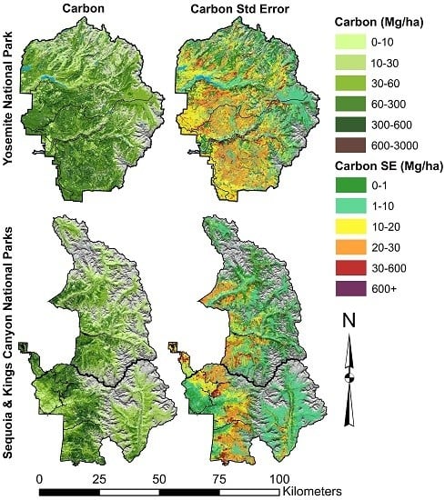
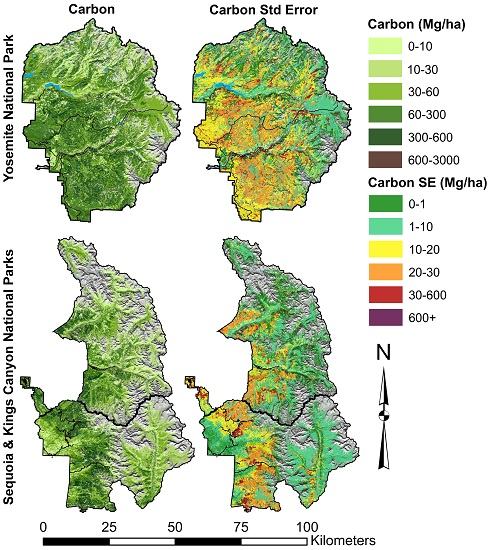
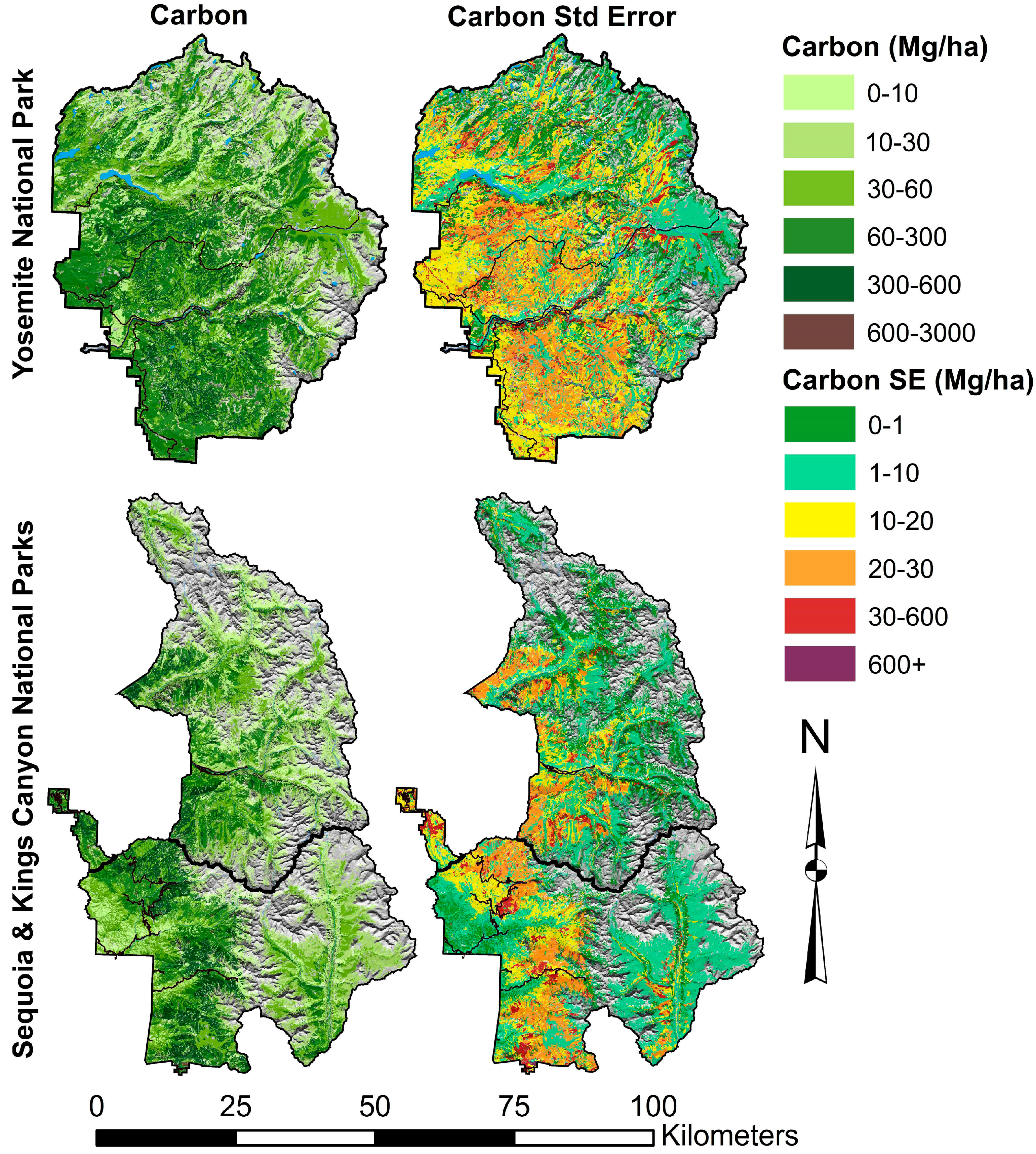
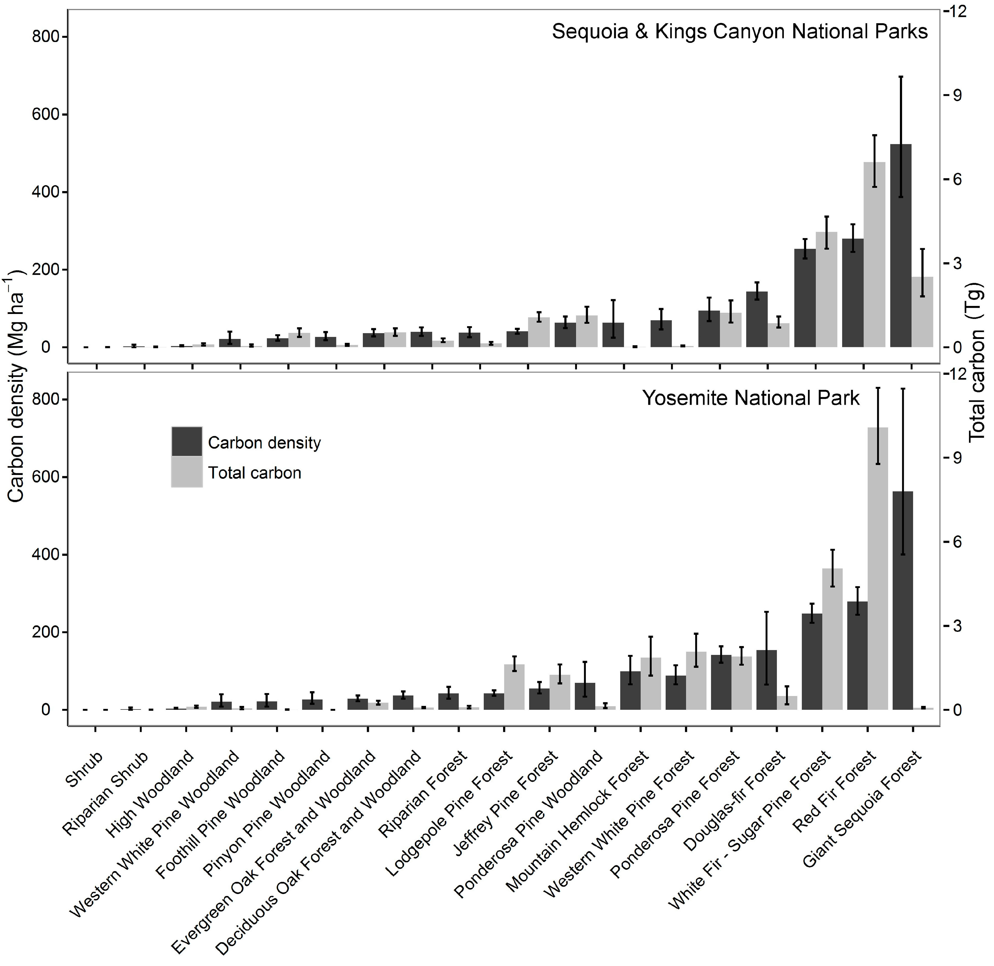
3.1. Aboveground Tree Carbon Stocks and Carbon Densities

We found that aboveground carbon in Yosemite was 25 Tg C (95% CI: 23–27 Tg C) and 20 Tg C for Sequoia (95% CI: 18–21 Tg C) (Figure 2).

Densities of aboveground tree carbon varied from a low of nearly 0 Mg·ha⁻¹ C in some shrub vegetation types to over 550 Mg·ha⁻¹ C in giant sequoia forests (Figure 3). Although the carbon densities for vegetation types were very similar between parks, the total carbon in many vegetation types differed substantially since the areal extents of the vegetation types differed (Figure 3). For example, in Sequoia, the namesake giant sequoia forests alone accounted for 10%–17% of total tree carbon, while in Yosemite, they accounted for 0.2%–0.4%. Red fir forest accounted for ⅓ of total tree carbon in both parks (37%–42% in Yosemite and 32%–36% in Sequoia), with Yosemite (8.8–11.5 Tg C) having nearly double the amount of carbon in its red fir than Sequoia (5.7–7.6 Tg C). White fir–sugar pine forests for both parks accounted for about 19%–22% of their respective total tree carbon (4.4–5.7 Tg C for Yosemite and 3.5–4.7 Tg C for Sequoia). Summaries of carbon by major forest types are shown in Figure 3 (see [41], Appendix C for detailed distributions).

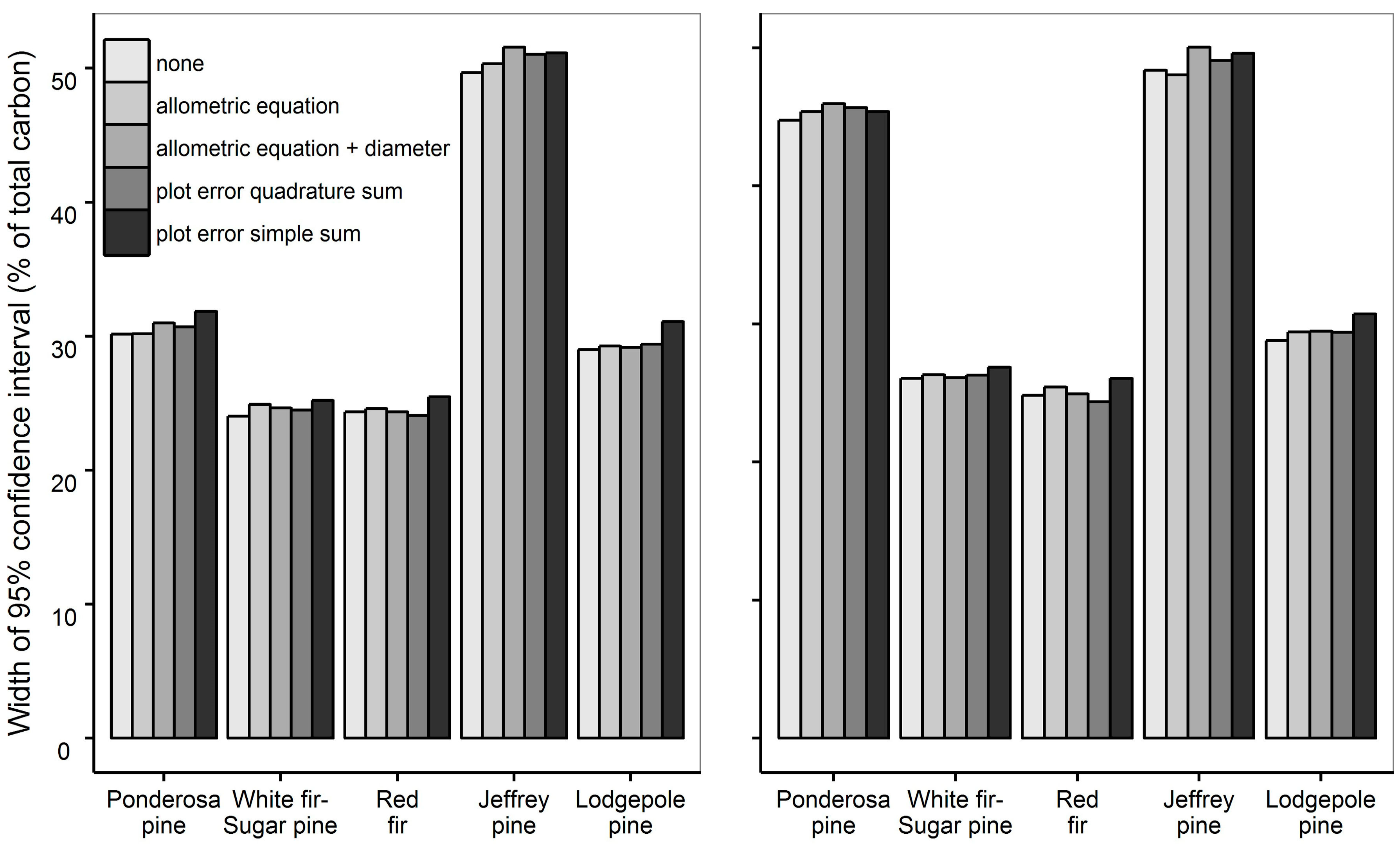
3.2. Carbon Uncertainties

We evaluated the relative contribution of five sources of error in carbon stock estimates, and found that in general, uncertainties associated with repeated measurements of tree diameters and allometric relationships had very little effect on the standard errors and confidence intervals of tree carbon density and total carbon estimates. The widths of the 95% confidence intervals for total carbon in several major forest types within both parks differed only slightly among the different methods of accounting for allometry error (Figure 4). The typical uncertainty arising from sampling a population—especially a very heterogeneous one—appears to be much more important for our dataset.

Forest type classification uncertainties, however, were an important component of uncertainty in total carbon estimates. We observed that Monte Carlo-estimated areas differed from observed mapped-based areas for several forest types. For example, a single summation of red fir forest polygons from Yosemite’s vegetation map yielded 41,315 ha, while the Monte Carlo estimate was 13% lower at 36,052 ha (95% CI: 34,655–37,723), suggesting that this forest type is over-mapped. Other forest types appeared to be under-mapped, for example, the high woodland type, which occurs on 26,602 ha in Yosemite according to the vegetation map, but was estimated by the Monte Carlo simulation to be 9% higher at 28,995 ha (95% CI: 28,307–29,953). These differences in area estimates noticeably affected total carbon estimates for some forest types, and usually widened the total carbon confidence intervals. Such differences, however, can also narrow the confidence intervals in some types (e.g., red fir) because the reduction in total area of the type leads to lower total carbon and confidence intervals generally become narrower as the estimate gets smaller.

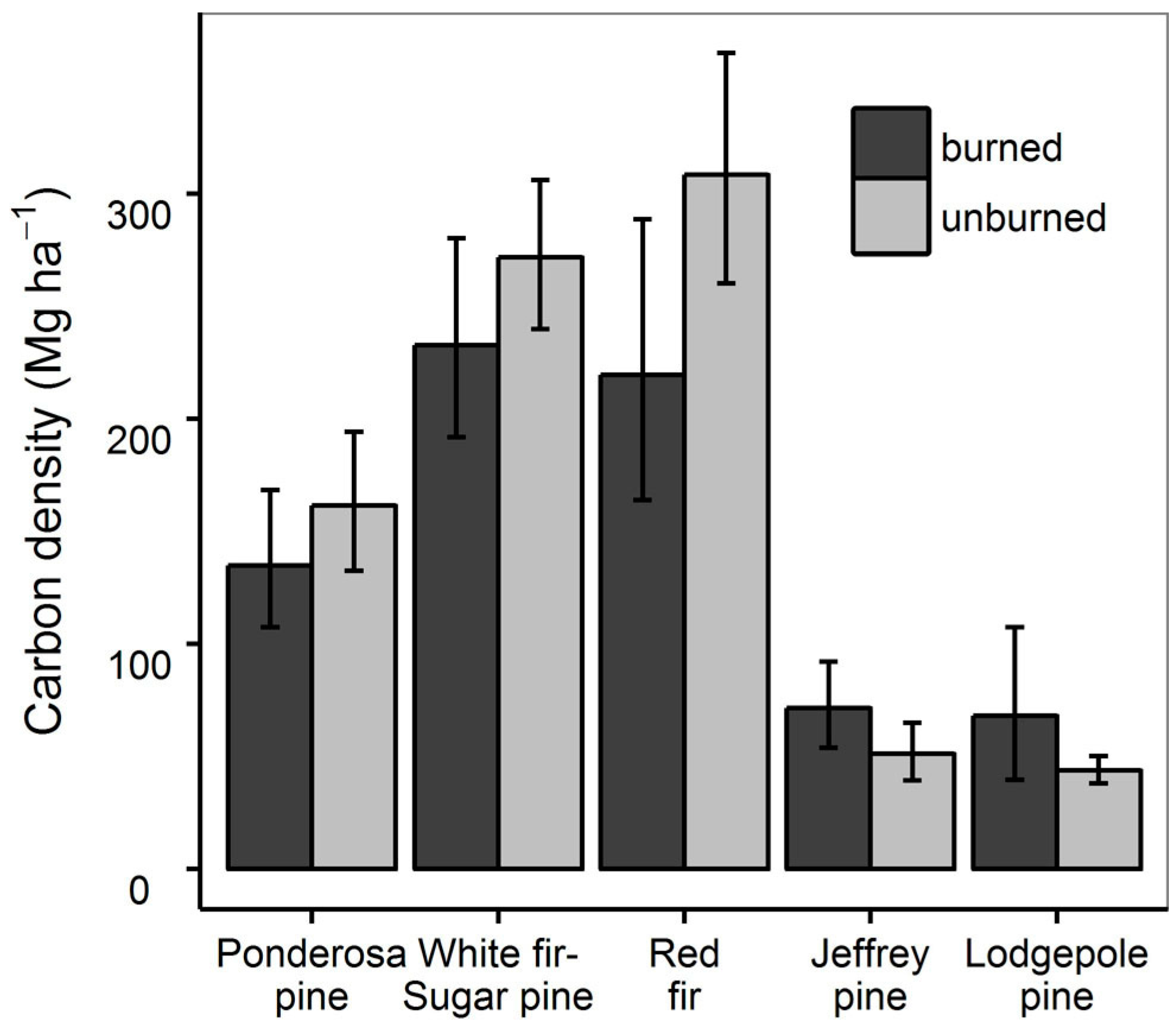
3.3. Fire History and Tree Carbon Density

The statistical model containing forest type, whether a plot was burned or unburned, and the interaction between burning and forest type had the greatest support (lowest AIC value) of our seven candidate models (

Table 2. Tree carbon density and fire history model comparisons for Yosemite and Sequoia & Kings Canyon National Parks.

Model Effects	AIC	ΔAIC
forest type	1698.6	2.97
forest type + burned	1699.6	3.93
forest type + burned + forest type × burned	1695.7	0.00
forest type + times burned	1700.6	4.96
forest type + times burned + forest type × times burned	1698.7	2.98
forest type + years since fire	1699.9	4.26
forest type + years since fire + forest type × years since fire	1696.7	1.01

). However, the statistical support for that model was only slightly greater than the model containing only forest type (AIC difference of ~3). The other candidate models using the other burn history metrics (number of times burned and years since most recent fire), either alone or interacting with forest type, did not have much support.

Aboveground tree carbon density estimates using the best model (forest type + burned + forest type × burned) indicated the burn history effect was inconsistent across forest types (Figure 5). The most substantial difference was in red fir forest, where carbon density was 29% lower if burned (absolute difference of 89 Mg·ha⁻¹ C; 95% CI: 4–169 Mg·ha⁻¹ C). Carbon densities were 15% lower in burned versus unburned within ponderosa pine (difference 26 Mg·ha⁻¹ C; 95% CI: −18–70 Mg·ha⁻¹ C) and white fir–sugar pine (difference 39 Mg·ha⁻¹ C; 95% CI: −18–94 Mg·ha⁻¹ C) forests. Jeffrey pine forests had 40% higher density within burned areas (difference 20 Mg·ha⁻¹ C; 95% CI: −2–44 Mg·ha⁻¹ C), and lodgepole pine forests also appeared to have slightly higher carbon density (difference 24 Mg·ha⁻¹ C; 95% CI: −6–63 Mg·ha⁻¹ C). The differences in carbon between burned and unburned for all but red fir forests included 0 within their 95% confidence intervals, and thus are not significant (Figure 5).

3.4. Carbon Stability and Future Fire

Our assessment of forest carbon at risk due to the period of fire absence found that 25 Tg C was contained within areas where the next fire is unlikely to be high severity and stand-replacing (FRID ≤ 1). Another 10 Tg C occurred in areas deemed moderately stable (1 < FRID ≤ 2.9). Approximately 5 Tg C were within areas considered with high probability to burn with substantial portions of high severity (FRID ≥ 3).

4. Discussion

We used an extensive ground-based plot dataset, the most applicable biomass allometry equations, and a robust statistical analysis to estimate aboveground tree carbon densities and total stocks, plus the uncertainty around those estimates, for Yosemite and Sequoia & Kings Canyon National Parks. Given these sources of uncertainty, most calculations of biomass or carbon can only give a range of biomass values—the combination of uncertainties is too large for a single number to be meaningful. This work has shown that even with thousands of calibration plots (e.g., [23]), there is still substantial uncertainty associated with quantifying carbon over the area of large landscapes. In fact, one of the most important results of this work may be the magnitude of the standard errors (±10%). Given the current state of allometric equations and vegetation classification, it may be impossible to make an estimate of carbon more precise than ±10%. Therefore, if policy proposals suggest a given treatment will change landscape carbon by less than 10%, there may be no practical way to evaluate the results.

Yosemite and Sequoia & Kings Canyon National Parks contain some of the largest individuals of Abies magnifica, Abies concolor, Pinus lambertiana, and Pinus jeffreyi [51] in addition to the largest individuals of Sequoiadendron giganteum. The biomass of these individuals is considerable (with densities of such trees generally 1 ha⁻¹ to 3 ha⁻¹), but no allometric equations extend to the diameters of the largest trees found in the monitoring plots or the surrounding forests. This required the use of proxy species, usually Abies procera and Pseudotsuga menziesii. Using allometric equations from proxy species is undesirable because of different bole taper, wood and bark densities and crown morphology. Inaccuracies due to proxy species are magnified in that allometric equations for large individuals only pertain to the tree bole. Although our methods did not reveal much error due to allometry, it was impossible for these methods (or any others) to ascertain the magnitude of error that could be present at tree diameters well above the maximums used to develop the allometric equations.

Small plot size and location may also influence carbon calculations. Most forest biomass resides in a small number (1% to 2%) of trees, and those trees may be distributed irregularly on the landscape [11,67]. Because the distribution and variability of biomass strongly depends on the spatial pattern of large-diameter trees [67,68,69,70], unbiased location of sufficient plot area is crucial to accurate calculations.

Though problematic from a computational and statistical standpoint, there is a growing body of literature suggesting that this skewed distribution toward large trees is a valuable and desired forest characteristic (e.g., [1,11,67,70] from a carbon, fire management, and a forest function perspective. For example, Lutz et al. [11] found that although large-diameter live trees (≥100 cm dbh) accounted for 1.4% of the individuals, they comprised 49.4% of total biomass in one Yosemite forest (white fir and sugar pine comprised 93% of large-diameter trees at their study site). Kane et al. [26] demonstrated that fires “thin from below” by removing much of the canopy area in the 2 to 8 m canopy strata. Thus, while fire removes biomass from forests, it disproportionately removes the understory at lower fire severity, leaving the large-diameter trees that contain a greater proportion of carbon. These large-diameter trees are perhaps the defining feature of these two parks. They are uniquely able to withstand all but the highest severity fires, and are of considerable ecological and social interest (including giving rise to the name of Sequoia National Park itself, and both parks have named individual stands of large trees). Dendro-chronological evidence confirms that these large trees developed under frequent fire regimes, with high severity fire patches limited in extent [38]. The resilience of large-diameter trees to damage from fires characteristic of the pre-suppression era suggests that their preservation is important to overall forest composition and structure, and most probably will continue to be so even under projected climate change scenarios [28].

This work focuses exclusively on standing live and dead tree carbon. Shrubs were excluded because of very few cover–biomass allometric equations available in the literature. Equations based on metrics such as basal stem diameter or crown diameter/height/volume are more common [12,34,71]. Unfortunately, none of those were measured for shrubs in the datasets we used. Shrub carbon usually accounts for a relatively small fraction of total aboveground carbon on landscapes dominated by trees. For example, shrub biomass within late-successional, lower mixed-conifer forests of the Sierra Nevada was approximately 1% of ecosystem biomass [11,12], and in early seral systems (those responding to high-severity fire in the study area), shrub biomass declined from about 33% of total biomass 20 years after stand-initiating disturbance to about 6% of total biomass 40 years later [34]. However, shrubs can be important to carbon cycling by fire; although representing only up to 4.5 Mg·ha⁻¹ in these forests [11], over 90% of shrub carbon can be consumed in even low- and moderate-severity fires [72]. We also excluded herbaceous (grasses, forbs, mosses, and lichens) biomass from our calculations, again due to a dearth of species-specific cover–biomass equations and low biomass with respect to trees [34].

Overall, our total YOSE tree carbon estimate of 25 Tg C is ~17% lower than the 2009 NASA-CASA estimate of 30 Tg C, and the NASA-CASA estimate is beyond the upper bound of our estimate’s 95% confidence interval (27 Tg C) [17]. The NASA-CASA estimates do not include errors, so it is difficult to judge the extent to which the two estimates differ, but there are a few possible reasons why differences should be expected. One potential underestimation in our method is that it excludes shrub biomass, as we were focused exclusively on tree carbon and unable to find adequate shrub cover–biomass allometry equations. In forests with older trees (~500 years) that have experienced frequent low-severity fire, shrubs constitute ~1% of total aboveground biomass, while shrub biomass can be a much higher percentage in stands that experienced high-severity fire [11]. When broken down by vegetation types, this difference is evident in the shrub and woodland vegetation categories, which might explain at least 2 Tg C of the difference between the two estimates, and brings a NASA-CASA estimate without shrubs (28 Tg C) very close to the upper end of our plot-based estimate (27 Tg C). However, the standard errors of our estimate are likely to be on the same order as the standard errors of the NASA-CASA approach. Should NASA-CASA include standard errors, there would likely be overlap between their estimates and ours.

In high elevation woodlands, NASA-CASA estimates fall well above ours. Inappropriate allometric equations may play a role. High elevation pines, especially those with larger diameters, are much more limited in their height at a given bole diameter when compared to low elevation pines. It is not uncommon for high elevation junipers and whitebark pines to have a dbh of 100 cm and a height less than 10 m. The baseline biomass calculations for NASA-CASA utilized generic pine allometric equations [17,18], and therefore almost certainly overestimate biomass of high elevation forests in the Sierra Nevada. We used equations based on arid juniper species [50], which have a height-constrained growth form similar to high elevation pines.

Our Yosemite carbon estimates are based on the vegetation map developed using aerial photography from 1997, and most of our field plots are from that time period. Unfortunately, NASA-CASA data are available for YOSE during only 2009, though eventually maps going back to 2000 will be produced [73]. Eleven years of tree growth between 1997 and 2009 may lead the NASA-CASA estimates to be higher than ours simply because of time, although a decade of change is probably still small with respect to the errors of the two estimates. Reconciling the two will require the use of established succession schemes [74], and the development of a downscaled NASA-CASA raster for the Yosemite (and potentially Sequoia) areas for the year 2000.

The current NASA-CASA scheme incorporates fire impacts on forest carbon stocks by assuming a reset back to a low, shrub-based value following a fire [17]. However, fires do not uniformly reduce carbon over the area within a fire perimeter—except in the most extreme high severity scenarios. Rather, there is a range of severities that produce a range of carbon loss to the atmosphere and transfer to the standing dead pool [31,75,76,77]. Figure 6 presents a basic model of carbon fluxes immediately following wildfire and provides a computational framework for post-fire carbon loss accounting using fire severity data. With this model, changes in carbon pools are calculated on a per-pixel basis, with pixels inferred as unburned (about 20% to 25% of the area within the fire perimeter), being assumed to have unchanged carbon pools [78,79,80,81,82,83]. Results from our carbon–fire history analysis—which showed only slight differences in carbon densities inside vs. outside fire perimeters—also support this notion of a mixed severity regime, where fire does not result in significant overall loss of carbon because large-diameter tree mortality is low. Fire typically produces a heterogeneous mix of carbon reductions, and the pattern of heterogeneity is indeed important for ecosystem functions such as vertebrate habitat creation [84]. Much of the carbon losses (at least in the low to moderate severity areas) is returned to the landscape by tree or shrub regeneration within a decade or two [80]. It is likely that an ecosystem carbon dynamics model which incorporates fire severity variables is better suited for quantifying responses in fire-prone landscapes, and would better compare contrasting fire management scenarios. We recommend a severity-based approach and illustrate its potential bias in the next section as a way to better quantify actual stock changes in fire-prone landscapes like Yosemite, and reconcile those changes with NASA-CASA remote sensing.

Using the scheme in Figure 6, remotely-sensed burn severity for the Rim Fire, and our tree carbon calculations, we estimate aboveground carbon in live tree biomass within the Rim Fire footprint in Yosemite was reduced from ~5 Tg C before the fire to ~4 Tg C after the fire, with ~1.4 Tg C as standing dead, and ~0.3 Tg C immediately lost to the atmosphere. NASA-CASA assumes a 100% loss of all pre-fire live and dead standing tree biomass. Our values are based on a hypothetical carbon loss by severity scheme, and we use this only as a means to illustrate the potential difference in estimated losses, not to provide definitive numbers for actual Rim Fire carbon losses. Measurements of ground-based plots and extended severity assessments one year after the fire will likely provide better estimates of responses in tree carbon pools to the Rim Fire.

Belowground carbon was excluded primarily because there are insufficient studies of total carbon in late-successional systems, especially those with large-diameter trees. Where total aboveground and belowground carbon pools and fluxes have been estimated [81], it has generally been the result of concentrated interdisciplinary research activity over many years [81]. Although fire removes large roots from previously dead trees and volatilizes some surface carbon, belowground stores of carbon are less changeable in response to fire than aboveground carbon. The importance of belowground carbon stocks implies a need for future research in this area.

The location of burned areas by fire perimeter alone did not yield significant differences between the carbon content of unburned and burned forests. However, the plot establishment scheme used in this study required forested plots (i.e., those with living trees). Therefore, ipso facto, plots with recent high-severity fire were not included. In addition, the burned versus unburned contrast in this study was for plots that were sampled with medians ranging from 14 to 16 years since last fire, with very few plots having >30 years since the last fire. Therefore, effects of fire at longer times since burning could not be addressed. However, these results do not suggest either a large or statistically significant effect of low- to moderate-severity fire. A more comprehensive assessment of the effects of fire on the landscape will require a consideration of fire severity [32,75], the proportionate area within a fire perimeter that remained unburned [78,79,82,83], and details on pre-fire and post-fire carbon accumulation rates [41,46,76].

5. Conclusions

The uncertainties associated with carbon calculations and the renewed emphasis on carbon inventories suggest that more emphasis needs to be placed on accurate landscape mapping and vegetation type classification. Many classification schemes rely on satellite-derived classifications, which are much less precise than the photointerpretation used here (e.g., 30 m pixels from Landsat vs. high resolution (<1 m) aerial photos). The collection of more extensive woody plant allometry data—a field of investigation generally out of favor since the 1980s—should be a priority, especially for large-diameter trees, which constitute a large and relatively unknown source of error. Similarly, priority should be given to large (≥1 ha) plots to reduce uncertainties related to the locations and patterns of large-diameter trees [69]. Finally, the immediate and delayed losses of tree carbon due to fire need more study given the uncertainties introduced by assumptions about consumption. No single method (including this one) can completely and definitively quantify tree carbon. However, given the current state of allometric equations and precision vegetation mapping, we did bound the uncertainty in carbon, and have provided a means for comparison with remote sensing techniques that can help update the map as carbon continues to accumulate and disturbances like fire alter baseline carbon densities. Combining these plot based methods for baselines and the tree coring work to calibrate pre- and post-fire recovery rates with remotely sensed carbon estimates is likely to provide the best way forward for managers to update carbon inventory maps.

The uncertainties in quantifying aboveground carbon in living and dead trees across landscapes suggest that inventories of carbon stocks, sequestration, and emissions, such as the California Air Resources Board Greenhouse Gas (GHG) inventory, may fail to reveal valuable estimates of carbon stocks, emissions or loss of carbon post wildfire. Land managers are increasingly asked to assess how restoration or vegetation treatment projects will impact climate change (e.g., 36 CFR 219.6b4; 2012 National Forest System Land Management Planning). Specifically, NEPA (National Environmental Policy Act) interdisciplinary (ID) teams are asked to evaluate how proposed fuel reduction treatments or revegetation/reforestation will effect GHG emissions and sequestration [85]. Such analyses would be more informative if they included the uncertainties of the carbon estimates. The uncertainties presented here suggest that NEPA analyses of the impacts that vegetation treatments (e.g., timber harvest, stand thinning, mechanical fuels treatments or prescribed fire) may have on climate change are limited in accuracy, particularly when treatment units contain trees larger than published allometries, carbon released to the atmosphere by fire is uncertain, and landscape-scale vegetation types are inconsistently defined. When errors in carbon calculations are considered, many proposed management alternatives may not differ statistically in their landscape-level carbon sequestration.

References

1. Hurteau, M.D.; Brooks, M.L. Short- and long-term effects of fire on carbon in US dry temperate forest ecosystems. BioScience 2011, 61, 139–146. [Google Scholar] [CrossRef]
2. Swann, A.L.S.; Fung, I.Y.; Chiang, J.C.H. Mid-latitude afforestation shifts general circulation and tropical precipitation. Proc. Natl. Acad. Sci. USA 2012, 109, 712–716. [Google Scholar] [CrossRef] [PubMed]
3. Smith, A.M.S.; Kolden, C.A.; Paveglio, T.B.; Cochrane, M.A.; Bowman, D.; Moritz, M.A.; Kliskey, A.D.; Alessa, L.; Hudak, A.T.; Hoffman, C.M.; et al. The science of firescapes: Achieving fire resilient communities. BioScience 2016, 66, 130–146. [Google Scholar] [CrossRef]
4. Becker, K.M.L.; Lutz, J.A. Can low-severity fire reverse overstory compositional change in montane forests of the Sierra Nevada, USA? Ecosphere 2016, 7, e01484. [Google Scholar] [CrossRef]
5. Chisholm, R.A.; Muller-Landau, H.C.; Abdul Rahman, K.; Bebber, D.P.; Bin, Y.; Bohlman, S.A.; Bourg, N.A.; Brinks, J.; Brokaw, N.; Bunyavejchewin, S.; et al. Scale-dependent relationships between species richness and ecosystem function in forests. J. Ecol. 2013, 101, 1214–1224. [Google Scholar] [CrossRef]
6. Larson, A.J.; Lutz, J.A.; Gersonde, R.F.; Franklin, J.F.; Hietpas, F.F. Productivity influences the rate of forest structural development. Ecol. Appl. 2008, 18, 899–910. [Google Scholar] [CrossRef] [PubMed]
7. Yanai, R.D.; Battles, J.J.; Richardson, A.D.; Blodgett, C.A.; Wood, D.M.; Rastetter, E.B. Estimating uncertainty in ecosystem budget calculations. Ecosystems 2010, 13, 239–248. [Google Scholar] [CrossRef]
8. Yanai, R.D.; Levine, C.R.; Green, M.B.; Campbell, J.L. Quantifying uncertainty in forest nutrient budgets. J. For. 2012, 110, 448–456. [Google Scholar] [CrossRef]
9. Chave, J.; Condit, R.; Aguilar, S.; Hernandez, A.; Lao, S.; Perez, R. Error propagation and scaling for tropical biomass estimates. Philos. Trans. R. Soc. Lond. B 2004, 359, 409–420. [Google Scholar] [CrossRef] [PubMed]
10. Harmon, M.E.; Fasth, B.; Halpern, C.B.; Lutz, J.A. Uncertainty analysis: An evaluation metric for synthesis science. Ecosphere 2015, 6. [Google Scholar] [CrossRef]
11. Lutz, J.A.; Larson, A.J.; Swanson, M.E.; Freund, J.A. Ecological importance of large-diameter trees in a temperate mixed-conifer forest. PLoS ONE 2012, 7, e36131. [Google Scholar] [CrossRef] [PubMed]
12. Lutz, J.A.; Schwindt, K.A.; Furniss, T.J.; Freund, J.A.; Swanson, M.E.; Hogan, K.I.; Kenagy, G.E.; Larson, A.J. Community composition and allometry of Leucothoe davisiae, Cornus sericea, and Chrysolepis sempervirens. Can. J. For. Res. 2014, 44, 677–683. [Google Scholar] [CrossRef]
13. Gabrielson, A.T.; Larson, A.J.; Lutz, J.A.; Reardon, J.J. Biomass and burning characteristics of sugar pine cones. Fire Ecol. 2012, 8, 58–70. [Google Scholar] [CrossRef]
14. Larson, A.J.; Cansler, C.A.; Cowdery, S.G.; Hiebert, S.; Furniss, T.J.; Swanson, M.E.; Lutz, J.A. Post-fire morel (Morchella) mushroom production, spatial structure, and harvest sustainability. For. Ecol. Manag. 2016, 377, 16–25. [Google Scholar] [CrossRef]
15. Saatchi, S.S.; Houghton, R.A.; Dos Santos Alvala, R.C.; Soares, J.V.; Yu, Y. Distribution of aboveground live biomass in the Amazon basin. Glob. Chang. Biol. 2007, 13, 816–837. [Google Scholar] [CrossRef]
16. Erickson, H.E.; Soto, P.; Johnson, D.W.; Roath, B.; Hunsaker, C. Effects of vegetation patches on soil nutrient pools and fluxes within a mixed-conifer forest. For. Sci. 2005, 51, 211–220. [Google Scholar]
17. Potter, C. The carbon budget of California. Environ. Sci. Policy 2010, 13, 373–383. [Google Scholar] [CrossRef]
18. Pan, Y.; Birdsey, R.A.; Fang, J.; Houghton, R.; Kauppi, P.E.; Kurz, W.A.; Phillips, O.L.; Shvidenko, A.; Lewis, S.L.; Canadell, J.G.; et al. A large and persistent carbon sink in the world’s forests. Science 2011, 333, 988–993. [Google Scholar] [CrossRef] [PubMed]
19. Jenkins, J.C.; Chojnacky, D.C.; Heath, L.S.; Birdsey, R.A. Comprehensive Database of Diameter-Based Biomass Regressions for North American Tree Species; USDA Forest Service General Technical Report 2004, NE-319; USDA Forest Service: Newtown Square, PA, USA, 2003. [Google Scholar]
20. Melson, S.L.; Harmon, M.E.; Fried, J.S.; Domingo, J.B. Estimates of live-tree carbon stores in the Pacific Northwest are sensitive to model selection. Carbon Balance Manag. 2011, 6, 2. [Google Scholar] [CrossRef] [PubMed]
21. Sillett, S.C.; van Pelt, R. Trunk reiteration promotes epiphytes and water storage in an old-growth redwood forest canopy. Ecol. Monogr. 2007, 77, 335–359. [Google Scholar] [CrossRef]
22. Van Pelt, R.; Sillett, S.C. Crown development throughout the lifespan of coastal Pseudotsuga menziesii, including a conceptual model for tall conifers. Ecol. Monogr. 2008, 78, 283–311. [Google Scholar] [CrossRef]
23. Wilson, B.T.; Woodall, C.W.; Griffith, D.M. Imputing forest carbon stock estimates from inventory plots to a nationally continuous coverage. Carbon Balance Manag. 2013, 8, 1. [Google Scholar] [CrossRef] [PubMed]
24. Morrison, K.D.; Kolden, C.A. Development of a historical multi-year land cover classification incorporating wildfire effects. Land 2014, 3, 1214–1231. [Google Scholar] [CrossRef]
25. Kane, V.R.; Gersonde, R.F.; Lutz, J.A.; McGaughey, R.J.; Bakker, J.D.; Franklin, J.F. Patch dynamics and the development of structural and spatial heterogeneity in Pacific Northwest forests. Can. J. For. Res. 2011, 41, 2276–2291. [Google Scholar] [CrossRef]
26. Kane, V.R.; Lutz, J.A.; Roberts, S.L.; Smith, D.F.; McGaughey, R.J.; Povak, N.A.; Brooks, M.L. Landscape-scale effects of fire severity on mixed-conifer and red fir forest structure in Yosemite National Park. For. Ecol. Manag. 2013, 287, 17–31. [Google Scholar] [CrossRef]
27. Kane, V.R.; North, M.; Lutz, J.A.; Churchill, D.; Roberts, S.L.; Smith, D.F.; McGaughey, R.J.; Kane, J.T.; Brooks, M.L. Assessing fire-mediated change to forest spatial structure using a fusion of Landsat and airborne LiDAR data in Yosemite National Park. Remote Sens. Environ. 2014, 151, 89–101. [Google Scholar] [CrossRef]
28. Lutz, J.A.; van Wagtendonk, J.W.; Franklin, J.F. Climatic water deficit, tree species ranges, and climate change in Yosemite National Park. J. Biogeogr. 2010, 37, 936–950. [Google Scholar] [CrossRef]
29. Lutz, J.A.; Halpern, C.B. Tree mortality during early forest development: a long-term study of rates, causes, and consequences. Ecol. Monogr. 2006, 76, 257–275. [Google Scholar] [CrossRef]
30. North, M.J.; Innes, J.; Zald, H. Comparison of thinning and prescribed fire restoration treatments to Sierran mixed-conifer historic conditions. Can. J. For. Res. 2007, 37, 331–342. [Google Scholar] [CrossRef]
31. Van Wagtendonk, J.W.; Lutz, J.A. Fire regime attributes of wildland fires in Yosemite National Park, USA. Fire Ecol. 2007, 3, 34–52. [Google Scholar] [CrossRef]
32. Lutz, J.A.; Key, C.H.; Kolden, C.A.; Kane, J.T.; van Wagtendonk, J.W. Fire frequency, area burned, and severity: A quantitative approach to defining a normal fire year. Fire Ecol. 2011, 7, 51–65. [Google Scholar] [CrossRef]
33. Hurteau, M.D.; North, M.P. Fuel treatment effects on tree-based forest carbon storage and emissions under modeled wildfire scenarios. Front. Ecol. Environ. 2009, 7, 409–414. [Google Scholar] [CrossRef]
34. Halpern, C.B.; Lutz, J.A. Canopy closure exerts weak controls on understory dynamics: A 30-year study of overstory-understory interactions. Ecol. Monogr. 2013, 83, 19–35. [Google Scholar] [CrossRef]
35. Van Wagtendonk, J.W.; Fites-Kaufman, J. Sierra Nevada bioregion. In Fire in California’s Ecosystems; Sugihara, N.G., van Wagtendonk, J.W., Shaffer, K.E., Fites-Kaufman, J., Thode, A.E., Eds.; University of California Press: Berkeley, CA, USA, 2006; pp. 264–294. [Google Scholar]
36. Fites-Kaufman, J.; Rundel, P.; Stephenson, N.; Weixelman, D.A. Montane and subalpine vegetation of the Sierra Nevada and Cascade ranges. In Terrestrial Vegetation of California; Barbour, M.G., Keeler-Wolf, T., Schoenherr, A.A., Eds.; University of California Press: Berkeley, CA, USA, 2007; pp. 456–501. [Google Scholar]
37. Kane, V.R.; Lutz, J.A.; Cansler, C.A.; Povak, N.A.; Churchill, D.; Smith, D.F.; Kane, J.T.; North, M.P. Water balance and topography predict fire and forest structure patterns. For. Ecol. Manag. 2015, 338, 1–13. [Google Scholar] [CrossRef]
38. Scholl, A.E.; Taylor, A.H. Fire regimes, forest change, and self-organization in an old-growth mixed-conifer forest, Yosemite National Park, USA. Ecol. Appl. 2010, 20, 362–380. [Google Scholar] [CrossRef] [PubMed]
39. Barth, M.A.F.; Larson, A.J.; Lutz, J.A. Use of a forest reconstruction model to assess changes to Sierra Nevada mixed-conifer forest during the fire suppression era. For. Ecol. Manag. 2015, 354, 104–118. [Google Scholar] [CrossRef]
40. Levine, C.R.; Cogbill, C.V.; Collins, B.M.; Larson, A.J.; Lutz, J.A.; North, M.P.; Restaino, C.M.; Safford, H.D.; Stephens, S.L.; Battles, J.J. Evaluating a new method for reconstructing forest conditions from General Land Office survey records. Ecol. Appl. 2017, in press. [Google Scholar]
41. Matchett, J.R.; Lutz, J.A.; Tarnay, L.W.; Smith, D.G.; Becker, K.M.L.; Brooks, M.L. Impacts of Fire Management on Aboveground Tree Carbon Stocks in Yosemite and Sequoia & Kings Canyon National Parks; Natural Resources Report, NPS/SIEN/NRR-2015/910; National Park Service: Fort Collins, CO, USA, 2015. [Google Scholar]
42. Keeler-Wolf, T.; Moore, P.E.; Reyes, E.T.; Menke, J.M.; Johnson, D.N.; Karavidas, D.L. Yosemite National Park Vegetation Classification and Mapping Project Report; Natural Resource Technical Report, NPS/YOSE/NRTR—2012/598; National Park Service: Fort Collins, CO, USA, 2012. [Google Scholar]
43. Aerial Information Systems, Inc. USGS-NPS Vegetation Mapping Program, Sequoia & Kings Canyon National Parks Photo Interpretation Report; Aerial Information Systems, Inc.: Redlands, CA, USA, 2007. [Google Scholar]
44. Stephens, S.L.; Lydersen, J.M.; Collins, B.M.; Fry, D.L.; Meyer, M.D. Historical and current landscape-scale ponderosa pine and mixed conifer forest structure in the southern Sierra Nevada. Ecosphere 2015, 6, 1–63. [Google Scholar] [CrossRef]
45. Van de Water, K.M.; Safford, H.D. A summary of fire frequency estimates for California vegetation before Euro-American settlement. Fire Ecol. 2011, 7, 26–58. [Google Scholar] [CrossRef]
46. Van Wagtendonk, J.W.; Moore, P.E. Fuel deposition rates of montane and subalpine conifers in the central Sierra Nevada, California, USA. For. Ecol. Manag. 2010, 259, 2122–2132. [Google Scholar] [CrossRef]
47. Means, J.E.; Hansen, H.A.; Koerper, G.J.; Alaback, P.B.; Klopsch, M.W. Software for Computing Plant Biomass—Biopak Users Guide; USDA Forest Service General Technical Report 1994, PNW-GTR-340; US Department of Agriculture, Forest Service, Pacific Northwest Research Station: Corvallis, OR, USA, 1994.
48. Westman, W.E. Aboveground biomass, surface area, and production relations of red fir (Abies magnifica) and white fir (A. concolor). Can. J. For. Res. 1998, 17, 311–319. [Google Scholar] [CrossRef]
49. Jenkins, J.C.; Chojnacky, D.C.; Heath, L.S.; Birdsey, R.A. National-scale biomass estimators for United States tree species. For. Sci. 2003, 49, 12–35. [Google Scholar]
50. Miller, L.M.; Meeuwig, R.O.; Budy, J.D. Biomass of Singleleaf Pinyon and Utah Juniper; USDA Forest Service, Intermountain Forest and Range Experimental Station Research Paper 1981, INT-273; Department of Agriculture, Forest Service, Intermountain Forest and Range Experiment Station: Ogden, UT, USA, 1981.
51. Van Pelt, R. Forest Giants of the Pacific Coast; University of Washington Press: Seattle, WA, USA, 2001. [Google Scholar]
52. Demaerschaulk, J.P.; Omule, S.A.Y. Estimating breast height diameters from stump measurements in British Columbia. For. Chron. 1982, 58, 143–145. [Google Scholar] [CrossRef]
53. Thomas, S.C.; Martin, A.R. Carbon content of tree tissues: A synthesis. Forests 2012, 3, 332–352. [Google Scholar] [CrossRef]
54. Lamlom, S.H.; Savidge, R.A. A reassessment of carbon content in wood: Variation within and between 41 North American species. Biomass Bioenergy 2003, 25, 381–388. [Google Scholar] [CrossRef]
55. Gonzalez, P.; Asner, G.P.; Battles, J.J.; Lefsky, M.A.; Waring, K.M.; Palace, M. Forest carbon densities and uncertainties from LiDAR, QuickBird, and field measurements in California. Remote Sens. Environ. 2010, 114, 1561–1575. [Google Scholar] [CrossRef]
56. Baskerville, G.L. Use of logarithmic regression in the estimation of plant biomass. Can. J. For. Res. 1972, 2, 49–53. [Google Scholar] [CrossRef]
57. R Core Team. R: A Language and Environment for Statistical Computing, Version 3.0; R Foundation for Statistical Computing: Vienna, Austria, 2013. Available online: http://www.R-project.org/ (accessed on 5 January 2013).
58. Wickham, H. Ggplot2: Elegant Graphics for Data Analysis; Springer: New York, NY, USA, 2009. [Google Scholar]
59. PostGIS Development Team. PostGIS, Version 2.1; 2013. Available online: http://postgis.net (accessed on 5 January 2013).
60. QGIS Development Team. QGIS, Version 2.4; 2013. Available online: http://qgis.net (accessed on 5 January 2013).
61. Kane, V.R.; Cansler, C.A.; Povak, N.A.; Kane, J.T.; McGaughey, R.J.; Lutz, J.A.; Churchill, D.J.; North, M.P. Mixed severity fire effects within the Rim fire: Relative importance of local climate, fire weather, topography, and forest structure. For. Ecol. Manag. 2015, 358, 62–79. [Google Scholar] [CrossRef]
62. Stavros, E.N.; Tane, Z.; Kane, V.R.; Veraverbeke, S.; McGaughey, R.J.; Lutz, J.A.; Ramirez, C.; Schimel, D. Unprecedented remote sensing data over the King and Rim megafires in the Sierra Nevada mountains of California. Ecology 2016, 97, 3244. [Google Scholar] [CrossRef] [PubMed]
63. Safford, H.D.; van de Water, K.M. Using Fire Return Interval Departure (FRID) Analysis to Map Spatial and Temporal Changes in Fire Frequency on National Forest Lands in California; USDA Forest Service Research Paper 2014, PSW-RP-266; United States Department of Agriculture, Forest Service, Pacific Southwest Research Station: Albany, CA, USA, 2014.
64. Hann, W.J.; Strohm, D.J. Fire regime condition class and associated data for fire and fuels planning: methods and applications. In Fire, Fuel Treatments, and Ecological Restoration; Omi, P.N., Joyce, L.A., Eds.; USDA Forest Service Rocky Mountain Research Station: Fort Collins, CO, USA, 2003; pp. 397–434. [Google Scholar]
65. Safford, H.D.; van de Water, K.M.; Schmidt, D. California Fire Return Interval Departure (FRID) Map, 2010 Version; USDA Forest Service, Pacific Southwest Region, and The Nature Conservancy: Albany, CA, USA, 2011. [Google Scholar]
66. Van Wagtendonk, J.W.; van Wagtendonk, K.A.; Meyer, J.B.; Painter, K.J. The use of geographic information for fire management planning in Yosemite National Park. Appl. Geogr. 2002, 19, 19–39. [Google Scholar]
67. Lutz, J.A.; Larson, A.J.; Freund, J.A.; Swanson, M.E.; Bible, K.J. The ecological importance of large-diameter trees to forest structural heterogeneity. PLoS ONE 2013, 8, e82784. [Google Scholar] [CrossRef] [PubMed]
68. Miller, J.D.; Collins, B.M.; Lutz, J.A.; Stephens, S.L.; van Wagtendonk, J.W.; Yasuda, D.A. Differences in wildfires among ecoregions and land management agencies in the Sierra Nevada region, California, USA. Ecosphere 2012, 3, 80. [Google Scholar] [CrossRef]
69. Lutz, J.A. The evolution of long-term data for forestry: Large temperate research plots in an era of global change. Northwest Sci. 2015, 89, 255–269. [Google Scholar] [CrossRef]
70. Lutz, J.A.; Larson, A.J.; Furniss, T.J.; Freund, J.A.; Swanson, M.E.; Donato, D.C.; Bible, K.J.; Chen, J.; Franklin, J.F. Spatially non-random tree mortality and ingrowth maintain equilibrium pattern in an old-growth Pseudotsuga-Tsuga forest. Ecology 2014, 95, 2047–2054. [Google Scholar] [CrossRef] [PubMed]
71. McGinnis, T.W.; Shook, C.D.; Keeley, J.E. Estimating aboveground biomass for broadleaf woody plants and young conifers in Sierra Nevada, California, forests. West. J. Appl. For. 2010, 25, 203–209. [Google Scholar]
72. Lutz, J.A.; Furniss, T.J.; Germain, S.J.; Becker, K.M.L.; Blomdahl, E.; Jeronimo, S.A.; Cansler, C.A.; Freund, J.A.; Swanson, M.E.; Larson, A.J. Shrub consumption and immediate community change by reintroduced fire in Yosemite National Park, California, USA. Fire Ecol. 2017, 13. [Google Scholar] [CrossRef]
73. Potter, C.; Dolanc, C. Thirty years of change in subalpine forest cover from Landsat image analysis in the Sierra Nevada Mountains of California. For. Sci. 2016, 62, 623–632. [Google Scholar] [CrossRef]
74. Davis, B.H.; Beck, J.; van Wagtendonk, J.W. Modeling fuel succession. Fire Manag. Today 2009, 69, 18–21. [Google Scholar]
75. Lutz, J.A.; van Wagtendonk, J.W.; Thode, A.E.; Miller, J.D.; Franklin, J.F. Climate, lightning ignitions, and fire severity in Yosemite National Park, California, USA. Int. J. Wildland Fire 2009, 18, 765–774. [Google Scholar] [CrossRef]
76. Hurteau, M.D.; North, M. Carbon recovery rates following different wildfire risk mitigation treatments. For. Ecol. Manag. 2010, 260, 930–937. [Google Scholar] [CrossRef]
77. Carlson, C.H.; Dobrowski, S.Z.; Safford, H.D. Variation in tree mortality and regeneration affect forest carbon recovery following fuel treatments and wildfire in the Lake Tahoe Basin, California, USA. Carbon Balance Manag. 2012, 7, 7. [Google Scholar] [CrossRef] [PubMed]
78. Kolden, C.A.; Lutz, J.A.; Key, C.H.; Kane, J.T.; van Wagtendonk, J.W. Mapped versus actual burned area within wildfire perimeters: characterizing the unburned. For. Ecol. Manag. 2012, 286, 38–47. [Google Scholar] [CrossRef]
79. Abatzoglou, J.T.; Kolden, C.A. Relationships between climate and macroscale area burned in the western United States. Int. J. Wildland Fire 2013, 22, 1003–1020. [Google Scholar] [CrossRef]
80. Hurteau, M.D.; Stoddard, M.T.; Fule, P.Z. The carbon costs of mitigating high-severity wildfire in southwestern ponderosa pine. Glob. Chang. Biol. 2011, 17, 1516–1521. [Google Scholar] [CrossRef]
81. Fahey, T.J.; Siccama, T.G.; Driscoll, C.T.; Likens, G.E.; Campbell, J.; Johnson, C.E.; Battles, J.J.; Aber, J.D.; Cole, J.J.; Fisk, M.C.; et al. The biogeochemistry of carbon at Hubbard Brook. Biogeochemistry 2005, 75, 109–176. [Google Scholar] [CrossRef]
82. Kolden, C.A.; Abatzoglou, J.T.; Lutz, J.A.; Cansler, C.A.; Kane, J.T.; van Wagtendonk, J.W.; Key, C.H. Climate contributors to forest mosaics: Ecological persistence following wildfire. Northwest Sci. 2015, 89, 219–238. [Google Scholar] [CrossRef]
83. Meddens, A.J.H.; Kolden, C.A.; Lutz, J.A. Detecting unburned islands within fire perimeters using Landsat and ancillary data across the northwestern United States. Remote Sens. Environ. 2016, 186, 275–285. [Google Scholar] [CrossRef]
84. Roberts, S.L.; van Wagtendonk, J.W.; Kelt, D.A.; Miles, A.K.; Lutz, J.A. Modeling the effects of fire severity and spatial complexity on small mammals in Yosemite National Park, California. Fire Ecol. 2008, 4, 83–104. [Google Scholar] [CrossRef]
85. USDA Forest Service, Climate Change Land Management & Project Planning. Available online: http://www.fs.fed.us/emc/nepa/climate_change/includes/cc_nepa_guidance.pdf (accessed on 25 January 2017).
86. Gower, S.T.; Vogt, K.A.; Grier, C.C. Carbon dynamics of rocky mountain Douglas-fir: Influence of water and nutrient availability. Ecol. Monogr. 1992, 62, 43–65. [Google Scholar] [CrossRef]
87. Gholz, H.L.; Grier, C.C.; Campbell, A.G.; Brown, A.T. Equations for Estimating Biomass and Leaf area of Plants in the Pacific Northwest; Oregon State University School of Forestry Research Paper; Oregon State University: Corvallis, OR, USA, 1979; Volume 41, p. 39. [Google Scholar]
88. Grier, C.C.; Logan, R.S. Old-growth Pseudotsuga menziesii communities of a western Oregon watershed: biomass distribution and production budgets. Ecol. Monogr. 1977, 47, 373–400. [Google Scholar] [CrossRef]
89. Brown, J.K. Weight and Density of Crowns of Rocky Mountain Conifers; USFS Research Paper; United States Forest Service: Ogden, UT, USA, 1978. [Google Scholar]
90. Gower, S.T.; Grier, C.G.; Vogt, D.J.; Vogt, K.A. Allometric relations of deciduous (Larix occidentalis) and evergreen conifers (Pinus contorta and Pseudotsuga menziesii) of the Cascade Mountains in Central Washington. Can. J. For. Res. 1987, 17, 630–634. [Google Scholar] [CrossRef]
91. Pearson, J.A.; Fahey, T.J.; Knight, D.H. Biomass and leaf area in contrasting lodgepole pine forests. Can. J. For. Resour. 1984, 14, 259–265. [Google Scholar] [CrossRef]
92. Johnston, R.S.; Bartos, D.L. Summary of Nutrient and Biomass Data from Two Aspen Sites in Western United States; USFS Research Paper 1977, INT-277:15; US Forest Service: Washington, DC, USA, 1997. [Google Scholar]
93. Coltrin, W.R. Biomass Quantification of Live Trees in a Mixed Evergreen Forest Using Biomass Diameter-Based Allometric Equations. Master’s Thesis, Humboldt State University, Arcata, CA, USA, 2010. [Google Scholar]
Figure 1. Consolidated vegetation types of Yosemite and Sequoia & Kings Canyon National Parks. Unvegetated areas, principally near the crest of the Sierra Nevada, are gray. The 105 plots established for this study are shown as black circles (burned) and white circles (unburned). Figure adapted from [4].
Land 06 00010 g001
Figure 2. Geographic distribution of carbon (left) and the uncertainty of carbon (right) in Yosemite and Sequoia & Kings Canyon National Parks.
Land 06 00010 g002
Figure 3. Aboveground tree carbon densities (dark grey; left scale) and total carbon (light grey; right scale) for vegetation types in Sequoia & Kings Canyon (top) and Yosemite (bottom) National Parks. Means and 95% confidence intervals are shown. Although giant sequoia has the highest carbon density of any forest type, the contribution to total landscape carbon is only ranked third in Sequoia and was less than most other forest types in Yosemite.
Land 06 00010 g003
Figure 4. Comparisons of uncertainties in total carbon estimates for five forest types in Sequoia & Kings Canyon (left) and Yosemite (right) National Parks. The higher level of errors in Jeffrey pine and ponderosa pine forest types suggests that methods for more accurately mapping these forest types is needed, and also that the results of management actions in these forest types will be more uncertain.
Land 06 00010 g004
Figure 5. Combined aboveground tree and snag carbon stocks for Yosemite and Sequoia & Kings Canyon National Parks by consolidated forest type.
Land 06 00010 g005
Figure 6. Scheme for changes in tree carbon in response to fire severity [41]. Areas inferred to be unburned (usually from Landsat-derived metrics) are assumed to have no changes in carbon, even though considerable loss of sub-canopy trees, shrubs, litter, and duff is possible in areas inferred to be unburned.
Land 06 00010 g006