
Exergy Dynamics of Systems in Thermal or Concentration Non-Equilibrium


1
Department of Mechanical and Aerospace Engineering, Sapienza University of Rome, 00184 Roma, Italy
2
Department of Mathematics and Physics, Università Degli Studi Roma Tre, 00146 Roma, Italy
*
Author to whom correspondence should be addressed.
Entropy 2017, 19(6), 263; https://doi.org/10.3390/e19060263
Submission received: 23 March 2017
/
Revised: 29 May 2017
/
Accepted: 2 June 2017
/
Published: 8 June 2017
(This article belongs to the Special Issue Work Availability and Exergy Analysis)
Abstract
:The paper addresses the problem of the existence and quantification of the exergy of non-equilibrium systems. Assuming that both energy and exergy are a priori concepts, the Gibbs “available energy” A is calculated for arbitrary temperature or concentration distributions across the body, with an accuracy that depends only on the information one has of the initial distribution. It is shown that A exponentially relaxes to its equilibrium value, and it is then demonstrated that its value is different from that of the non-equilibrium exergy, the difference depending on the imposed boundary conditions on the system and thus the two quantities are shown to be incommensurable. It is finally argued that all iso-energetic non-equilibrium states can be ranked in terms of their non-equilibrium exergy content, and that each point of the Gibbs plane corresponds therefore to a set of possible initial distributions, each one with its own exergy-decay history. The non-equilibrium exergy is always larger than its equilibrium counterpart and constitutes the “real” total exergy content of the system, i.e., the real maximum work extractable from the initial system. A systematic application of this paradigm may be beneficial for meaningful future applications in the fields of engineering and natural science.
1. Introduction
1.1. Definition of Scope
This paper presents a derivation of the value of exergy for systems out of equilibrium. Our primary scope is to show that the calculation of the exergy of a non-equilibrium system is—under certain very general assumptions—possible without numerical approximations (both the diffusion and the thermodynamic equations can be solved analytically). The common idea is that exergy, being a function of state, can be calculated only in equilibrium transformations, following the usual quasi-equilibrium assumption: since obviously most processes of interest in engineering sciences are non-equilibrium ones, our approach is aimed at overcoming some of the inherent difficulties by taking an alternative point of view. Exergy has a property that neither energy nor entropy display: it quantifies directly the irreversibility in a process in an absolute and relative sense. An energy analysis does not take into account the different “quality” of the streams participating to a process, because it does not take into account their “convertibility” into useful work: here, exergy is superior. An entropy analysis, on the other hand, accurately quantifies the irreversibility, but without any reference to their relevance to the energy amount involved in the conversion or exchange. In other words, knowing the T0 is not sufficient information if we do not know how high is the involved Δh. Our approach calculates the entropy from the difference between energy and the exergy involved in the process, with the introduction of a standard (classical) equilibrium temperature T0. The energy (Δh) involved is known once the type of process is specified, and the exergy is calculated via constitutive evolution equations. Once it is accepted that exergy—under the abovementioned assumptions—is well-defined and measurable for systems far from equilibrium, it follows that if, as it is frequently the case, the energy of a system is known, a non-equilibrium entropy can be derived which reduces in the limit to the standard definition when the initial system is in equilibrium.
The procedure is based only on physical and classical first-order thermodynamic reasoning (heat and mass diffusion laws), and no new axiom is invoked: as such, it may be classified as a Classical Irreversible Thermodynamics method. It is presented here for a continuum, but an extension to finite ensembles of interacting particles is possible. Even if the procedure implies the local equilibrium assumption, its degree of theoretical accuracy is perfectly satisfactory.
The possibility of extending the definition of exergy to encompass non-equilibrium states is of great interest in at least two important scientific fields, namely engineering and environmental sciences. Process and component designers are very well aware that several engineering processes are not amenable to a classical equilibrium description because their evolution is poorly described by the “infinite series of quasi-equilibrium transformations” postulated by equilibrium Thermodynamics. Even excluding phenomena characterized by a high Knudsen number or by extremely short timescales, more common cases like the expansion of a real fluid in a turbine, separation by filtration, distillation, etc. display an intrinsic non-equilibrium character that forces designers to introduce empirical corrections into their phenomenological model, because no expansion is really adiabatic, no filtration really homogeneous, no distillation really single-phase. If the description of such processes could rely on a set of primitive thermodynamic variables known to maintain their validity under non-equilibrium conditions, their quantitative calculation could be improved and result in better designs. In environmental studies, non-equilibrium conditions are the rule: biologists, climatologists and environmentalists are concerned with systems that, from the very small to the very large, exist only in non-equilibrium conditions. The analysis of chemical processes in cells [1], atmospheric cycles [2] and complex living and non-living systems [3,4,5,6,7,8,9] would be simpler if globally valid non-equilibrium quantities were at hand. Most of these references present a different approach to the problem of defining a non-equilibrium entropy. They are all well-posed, and we do not imply that there is an error in the respective formulations: we simply claim that our approach is simpler and leads (for macroscopic systems) to accurate results with less effort. For example, the “entropy cascade” postulated in [10] leads indeed to a possible optimization, but is obtained once again in a lumped form: the distribution of T inside of the body or system is unspecified. Furthermore, Badescu’s procedure requires two steps that are absent in our formulation: first, the hierarchy of the levels must be identified and described; second, the respective influence coefficients must be calculated. Our approach disposes of both steps, retaining only the local equilibrium hypothesis, and is therefore much simpler to apply to real cases. In [11], the result is correctly recovered that the exergy destruction density is proportional to the irreversible portion of the entropy generation density: under equilibrium conditions, this is the Gouy–Stodola theorem. We “recover” the conclusion indirectly, in that we quantify the time evolution of the exergy of a system, and thus the total exergy destruction between two arbitrary states. As for [12,13], it is likely that their peculiar choice of the control volume affects the exergy budget: in the presence of a non-isothermal boundary, exergy fluxes may flow through the body, and either the system is in a dynamical steady state (similar to the pin in Section 8.3), or the discharged exergy fluxes do contribute to the time evolution of the system and in this case ought to be rigorously accounted for (i.e., separately from the exergy destruction). Finally, the distinction between reversible and “invertible” processes introduced in [14] has scientific merit, but their method is very much distant from what we propose.
1.2. Putting the Proposed Approach into Perspective
Classical Thermodynamics deals with systems “in equilibrium”, where this definition implies that the system (solid or fluid, simple or composite, continuous or discrete) is in a certain constrained state, completely described by a set of measurables called state variables, such that the values of these variables remain the same forever: no internal changes, or mass or energy exchanges with other systems are allowed. For added generality, we are including here the so-called steady-state processes, which are dynamic in the sense that, while mass and energy flows through their boundaries are allowed, they are treated under the assumption that the average (large-grain) conditions of all participating media remain unchanged in time. In fact, “time” is not a variable in equilibrium thermodynamics, so much so that renaming it “Thermostatics” was actually suggested in the past [15]. In nature and in the real world of engineering applications, an equilibrium system is a long shot exception rather than the rule: and even if we were capable of detecting and describing one such system, the slightest modification of the constraints (removing a rigid or an adiabatic partition, for example) would generate mass and/or energy exchanges within the system that can be described only in terms of time-dependent processes. Strictly speaking, even measuring the temperature of a finite-mass system with a thermometer may affect the state of the original system if the mass of the thermometer is not negligible with respect to that of the system (this applies to biological systems as well, see below). Notice though that our approach does not require the definition (or the calculation) of a “non-equilibrium temperature”. The reference temperature T0 is the equilibrium temperature of the immediate surroundings of the body under consideration. Thus, to extend equilibrium thermodynamics into the realm of real processes, the concepts of quasi-equilibrium and quasi-reversible process are customarily used: it is assumed that a system evolves in time from one state to the other through a (infinite) series of very small “changes”, such that: (a) the intermediate states can be represented on an equilibrium state diagram; (b) the integral along the path produces finite amounts of thermal and/or mechanical and/or chemical effects on the system and on other systems it may interact with.
This is an approximation, of course, but a very successful one, and it has led to a better understanding of real processes and to a vast body of theoretical knowledge resulting in innumerable successful applications to design and analysis issues in all engineering fields.
The discrepancy between the “ideal, equilibrium” behavior and that of the real system is handled by introducing numerical corrections into the model by means of properly defined coefficients that go under the name of “efficiencies”: thus, the expansion in a turbine necessarily generates less work than the “ideal one”, and the ηturbine < 1 accounts also for this “loss”. However, it is clear that a portion of the “work loss” in an expansion is due to non-equilibrium effects, like in undercooling or condensation effects in steam turbines, and to time-dependent mixing, like in desalination processes and deaerators. Similarly, the thermal energy subtracted to the hotter fluid in a heat exchanger cannot be completely recovered in the colder fluid, and the value of the heat exchanger effectiveness ε < 1 reflects also this imbalance. We say that, since energy is on the whole conserved, the “lost work” is converted into “irreversible entropy generation” causing a shift of a portion of the “ideal” work (or heat) towards the smaller scales of the participating media and thus an increase of the temperature of the final (again, equilibrium) state of the fluid. To provide a rigorous basis to the concept of efficiency, the irreversible entropy generation rate, which is a function of the fluxes, must be calculated, and Irreversible Thermodynamics was created to deal with this issue [15,16,17]. As an additional complication, time being now the essence of the “evolution” of the system from its initial to its final state, it is necessary to consider the different timescales spanned by the process, and since each scale may have its own energy budget, the calculation of the actual system evolution becomes intractably complicated [18].
Exergy is per se a good indicator of the degree of irreversibility in a process [19] hence the idea of using it to describe the evolution of a system in the non-equilibrium domain is appealing. However, though Gibbs’ original definition of Available Energy clearly envisioned a “relaxation process” from a non-equilibrium state to an equilibrium one through which some energy could be made “available”, no systematic treatment of the concept of non-equilibrium exergy can be found in the literature, and in fact there is no general agreement on the existence of such a quantity: scope of this paper is to clarify the issue and show that exergy is—under a proper set of assumptions—a quantity defined equally well for equilibrium and non-equilibrium systems. It is perhaps not superfluous to underscore though that we are not interested in providing a “new” definition of the exergy of non-equilibrium systems: the question we address is really “how much work can we extract from the evolution of a system from arbitrary initial conditions to its equilibrium state”, or, reversing the problem, “how much exergy must be supplied to a system initially in equilibrium to bring it to a specified non-equilibrium state”.
2. Two Necessary Primitives: Energy and Exergy
Consider an arbitrary system P of mass M known to be in a state P(t = 0) of non-equilibrium. If the analysis addresses only scales sufficiently removed from the smallest ones (those identified by statistical mechanics behavior), and if the gradients of the relevant measurables remain bounded throughout the system, we can divide P(t = 0) in a finite number k of spatial domains δPj such that , each one small enough to be considered in local equilibrium within the timescales imposed by the evolution of P: notice that this assumption, often criticized by theoreticians as lacking of rigor for its being clearly an approximation of reality, is currently a standard and very successful procedure adopted in numerical calculations of structural, thermal and fluid-dynamic processes (finite-elements, finite-volumes techniques). Each one of these domains has a measurable energy (cpjmjTj if thermal, 0.5mjVj2 if kinetic, etc.) and thus both the total and the specific energy of P at the time we open our window of observation are computable as well:
At any other instant τ, if it is possible to identify another finite number m, not necessarily equal to k, of spatial domains, each one still small enough to be considered in local equilibrium within the prevailing timescales between t = 0 and t = τ, the energy of the (closed) system is:
Since the time interval is arbitrary, as long as the above formulated local equilibrium assumption is acceptable, the evolution of the energy of the system is:
where dU/dt denotes the “infinitesimal” (continuous or finite) variation in time of the system’s energy.
If P is also isolated, then U(t) = U(0) at any time, and the evolution shall consist of a redistribution of the energy among the small spatial subdomains in which P is divided at each time. If P can exchange energy with the external world, then dU/dt is dictated by the prevailing boundary conditions.
3. Availability and Exergy
According to the original definition by Gibbs [20], the available energy or availability A is a thermodynamic function representing the maximum work that can be extracted from a system that proceeds from an initial arbitrary state to its final “internal” equilibrium state (i.e., the one attained while isolated from its surroundings). No restraint is imposed on the initial state of the system, and no interaction with the environment is postulated except for an ideal “available energy” release [21,22]. Under the assumptions posited in the previous section, each subdomain j of P has a perfectly computable (or measurable) available energy. Since the final state is an equilibrium one (same p, T, V, c, etc., for any j), the total availability of the initial state is:
Notice that the available energy is per se not additive: each subdomain J possesses at each instant of time 0 < t < τ an available energy aJ that depends on the “distance” of J from the system final “internal” equilibrium state. The system is in internal equilibrium, though not necessarily at its dead state, at time τ: if we introduce now the possibility that P(t = τ) interacts with an external reference environment, its exergy is classically defined as the maximum work that can be extracted from this exclusive interaction:
where the sum has been maintained to signify that now the interactions may also take place at the boundary, and some internal non-uniformity (gradient of some or all of the thermodynamic quantities throughout P) necessarily appears. Since, at time τ, although is in P equilibrium, the “classical” definition of exergy is valid for the entire system. Extending the above reasoning to initial non-equilibrium states, the non-equilibrium exergy of P(t = 0) can then be defined as:
Notice that the quantity defined by Equation (7) is always larger than the equilibrium exergy (Equation (6)), and is equal to the available energy only in the very special case in which the state of equilibrium of the isolated system is identical to the reference state (this is called the “dead state” in exergy jargon). When studying the evolution of non-equilibrium systems, Equation (7) rather than (5) or (6) should be applied.
Notice that the terms ej in (7) can also be computed directly, considering the evolution of each j-th subdomain from its initial local state δPj(t = 0) to its final dead state δPj(t = tfin) = (p0, T0, c0, V0, etc.). Notice also that when using Equation (6) or (7) a complete specification of the reference state AND of the boundary conditions must be provided.
4. Macroscopic Entropy as a Function of Energy and Exergy
The entropy of the system can be computed from the definition of exergy (E = U − T0S):
Equation (8) is—under the present assumptions—the non-equilibrium extension of the same formula derived for equilibrium systems by Haftopoulos and Gyftopoulos [23,24,25] and Gyftopoulos and Beretta [26]. It is worth mentioning that a completely opposite point of view exists [27,28], according to which it is possible to postulate the existence of a quantity called “non-equilibrium entropy” and derive Equation (8) as a corollary. As remarked by one of the Reviewers, Equation (8)—if taken by itself—may be seen as a postulate. However, in the present context, it is solely an extension of the definition of exergy, and it is justified by recalling that the original definition given by Gibbs to his Availability function was formulated for systems initially out of equilibrium. We wish to underline however that the purpose of the present paper is to compute the non-equilibrium exergy, and the fact that it may be used to compute a non-equilibrium entropy is an important corollary, but does not represent a fundamental issue in our approach. While we propose that formula (7) may represent a good definition of entropy for systems outside equilibrium, and will present some discussion in a later paper, nevertheless this must be viewed only as a consequence of the calculation of an exergy value for any state of non-equilibrium in which the initial conditions are exactly known.
5. Non Equilibrium Available Energy and Exergy in Solids
We consider a given spatially distributed mass with an initial temperature distribution and assume that the temperature evolves according to the Fourier law. The distribution of the mass can be one-, two- or three-dimensional. We shall refer in general to the mass distribution as “the solid”.
The Fourier model for the heat conduction equation in solids with convective boundary conditions reads
where is the temperature of the environment, is the thermal diffusivity, is the boundary of the solid, is the outward normal to the boundaries of the solid and is a measure of the heat transfer by convection at the boundaries of the solid.
We remember that the available energy is the maximum work that can be extracted from a system that proceeds from an initial arbitrary state to its final internal equilibrium state (the crucial point is that the body must be isolated from its surroundings). It is well known that the maximum work associated to a heat transfer from a temperature to a temperature is . In our case is the final internal equilibrium state (see Equation (11) below). Due to our assumption of local equilibrium, is the local temperature at the point at time t of the solid. The contribution from a small element to the availability is then given by
where (J/K) is the heat capacity of the solid and is the final equilibrium temperature distribution (notice that Equation (10) is, in this context, exact, since it follows directly from Gibbs’ definition, under the assumption of local equilibrium). Since, by definition, there is no exchange with the environment, we must set in Equation (9). Then the equilibrium temperature is found to be
where the integral must be performed over the volume (or surface, or curve) V occupied by the solid.
Note that can be also written, for any fixed , as the differential of , i.e.,
Our treatment can be generalized—with some mathematical complication—for variable density and specific heat distributions within the solid. However, in the remaining of this paper we will stipulate that and c, and thence , are constant throughout the solid. If the equilibrium temperature is taken as a reference, integrating Equation (10) from the actual temperature of the solid at and , , to the reference temperature , the contribution to the available energy is given by
The contribution from the entire solid at time t is found by integrating over the volume (surface/curve, respectively) and taking the difference between the available energy at time 0 and the available energy at time t:
where we assume for simplicity’s sake that both the specific heat capacity and the material density remain constant throughout. By taking into account the conservation of energy in the insulated solid, that is
we obtain
and the total available energy is found by taking the limit , that is
For the calculation of the exergy of the solid as a function of time, we must take the environment temperature as reference. In addition, in the system of Equations (9), we must consider a value of different from zero, to account for a thermal exchange between the solid and the environment. By a line of reasoning similar to the one adopted above, we derive the contribution from each particle of solid at location and time :
By integrating the previous expression from the actual temperature of the bar at and t, , and the reference temperature , the local contribution to the exergy is given by
The instantaneous contribution from the entire solid at time is found by integrating over the domain of interest, that is
where the cumulative amount of exergy destroyed at time in the process is found by the difference between the exergy at time 0 and the exergy at time t. We obtain:
and the total non-equilibrium exergy is found by taking the limit in :
In this formula, is the final distribution of temperature: if the boundary conditions are described by Equation (9) (i.e., the solid is immersed in an environment at constant temperature ) then is constant and equal to .
The classical equilibrium exergy of the system is given by
Recalling that = , the difference between the non-equilibrium exergy and the classical exergy can be written, in the case of an environment at constant temperature, as:
The quantity defined by Equation (24) is always nonnegative (this follows directly from Jensen’s inequality for concave functions). Thus, we can conclude that the non-equilibrium exergy (Equation (22)) is always greater than (or at most equal to) the classical exergy (Equation (23)).
Let us make a last remark: if the steady state of the solid is a state of non-equilibrium, that is if temperature gradients on the surface of the solid still exist for t → ∞, convective heat exchanges will also take place at large times. This can happen when the temperature on the boundaries of the solid is not uniform: for example a portion of the solid is in thermal contact with a bath at T1 and another portion exchanges heat by convection with the environment at T0: under these circumstances the exergy of the system will assume a constant value—different from zero—for . An example is given in Section 6. In such cases, it is more convenient to analyze the evolution of the irreversible exergy destruction inside of the solid: this point will be clarified in the next section.
6. A Non-Conservative Evolution Equation for Exergy
Associated with the temperature flow inside the solid there is an exergy current. This is equivalent to state that the exergy formally satisfies a non-conservative balance equation: let us discuss this point. In the absence of an internal source, the derivative of the specific exergy with respect to , at any point in the solid, is
where we used and . Equation (25) follows directly from the assumptions of local equilibrium and of validity of the Fourier diffusion law. If another constitutive equation (e.g., Cattaneo’s) is taken instead, will take a corresponding-different-form. The previous expression can be also rewritten as
If we identify the exergy flux by ( is the heat flux), the balance equation becomes:
where is the rate of exergy destruction per unit volume inside the solid. This term is negative definite, as it must be, because the Second Law imposes that the rate of time change in E be always smaller than the exergy inflow through the surface of the system and always larger than the exergy outflow through that surface. From Equation (27) we see that—in a physical sense—there is no “exergy balance”: a portion of the influx is unavoidably destroyed by irreversibility. The total exergy destruction at time is
As for the entropy balance equation, the exergy decrease of the system can be divided in two parts: one () is due to interactions with the environment, while the other accounts for the irreversible changes inside the system. Notice that is related to the entropy production rate inside the solid by . For a discussion about the evolution and the properties of the entropy production rate due to irreversible changes inside the system see [29,30].
7. Non Equilibrium Exergy in Mass Transfer Processes
In this section, we consider a given initial distribution of a liquid or a gas diffusing in a region under a difference of concentrations (chemical potential). We assume that the diffusion process is described by Fick’s law.
The initial spatial distribution of concentration (number of molecules per unit of volume) in the region is a given function and can be one-, two- or three-dimensional. We shall refer in general to this distribution as “the fluid”. The surrounding has a constant concentration equal to and a constant temperature T. In the case of impermeable boundary conditions, the system shall evolve towards a uniform equilibrium concentration , given by
Let us calculate the time history of the exergy of the system. We must allow for an exchange of mass at the permeable boundaries: the contribution of the mass in to the variation of exergy at time is proportional to the chemical potential of the substance in at times the variation of the number of molecules in the region considered, i.e., . Indeed, since the temperature is constant throughout the body, there is no heat flow, but under the imposed b.c. there is a mass flow: the previous equation then provides, under the hypothesis of local equilibrium, a quantitative measure of the exergy content of this flow. In a completely similar way as for heat transfer processes, a corresponding value of non-equilibrium exergy may thus be derived. As the reference state for the chemical potential, we take the environmental constant concentration . The chemical potential is given by , where is the activity of the substance. The concentration is related to the activity by an activity-coefficient that we assume to be constant, so we can write [8] .
If is a small region around , the contribution in at is
Since we take as reference the concentration , the contribution of the parcel dx to the exergy of the domain is obtained by integrating Equation (30) from the concentration of the fluid at and to the reference concentration:
The instantaneous contribution from the entire fluid at time is found by integrating over the volume (surface/line, respectively)
where the total amount of exergy at time t is found by making the difference between the exergy at time 0 and the exergy at time t:
The total non-equilibrium exergy is found by taking the limit of Equation (33):
The classical equilibrium exergy of the system is given by
The difference between the non-equilibrium exergy and the classical exergy can be written as
The above quantity is strictly non-negative (this follows again from Jensen’s inequality for convex functions). Hence, we conclude that the non-equilibrium exergy (Equation (34)) is always greater than (or at least equal to) the classical exergy (Equation (35)).
We can repeat the above derivation to find the expression of the available energy. In this case, we must consider impermeable boundary conditions. The available energy at time t is be given by
where we used the conservation law . The total available energy is found by taking the limit for t → ∞:
In the next section, we provide examples of calculation of the non-equilibrium exergy for some physical systems of interest.
8. Five Examples of Non-Equilibrium Systems with Computable Exergy
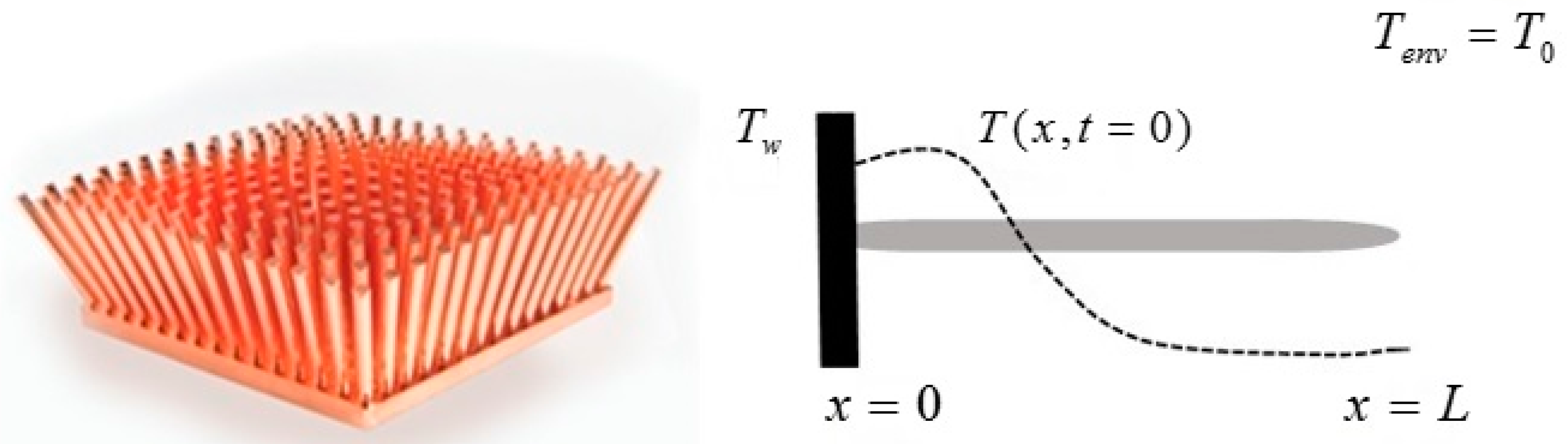
8.1. A Solid Bar with Initial Uneven Temperature Distribution
Consider a slender homogeneous metallic bar of length L and cross section A = s2, with so that the problem may be treated in a one-dimensional approximation: the prismatic surface of the bar is adiabatic and thermal energy can only be exchanged with the environment at the bar ends, x = 0 and x = L. The initial temperature distribution is . The surrounding is at T0. The temperature evolves according to Equation (9) and an explicit formula can be obtained for through a Fourier series expansion.
As a first case, consider an initial parabolic profile above or below the equilibrium temperature, that is
If we scale the temperature with , that is we set , then
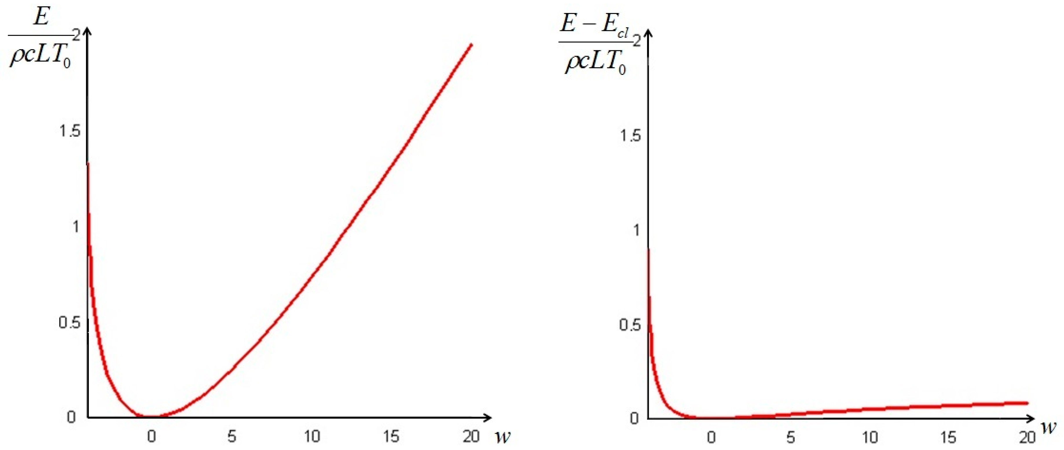
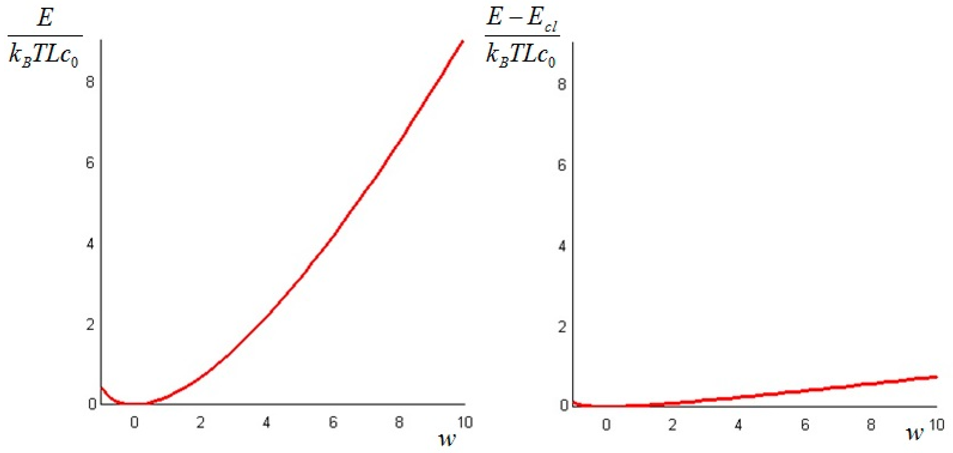
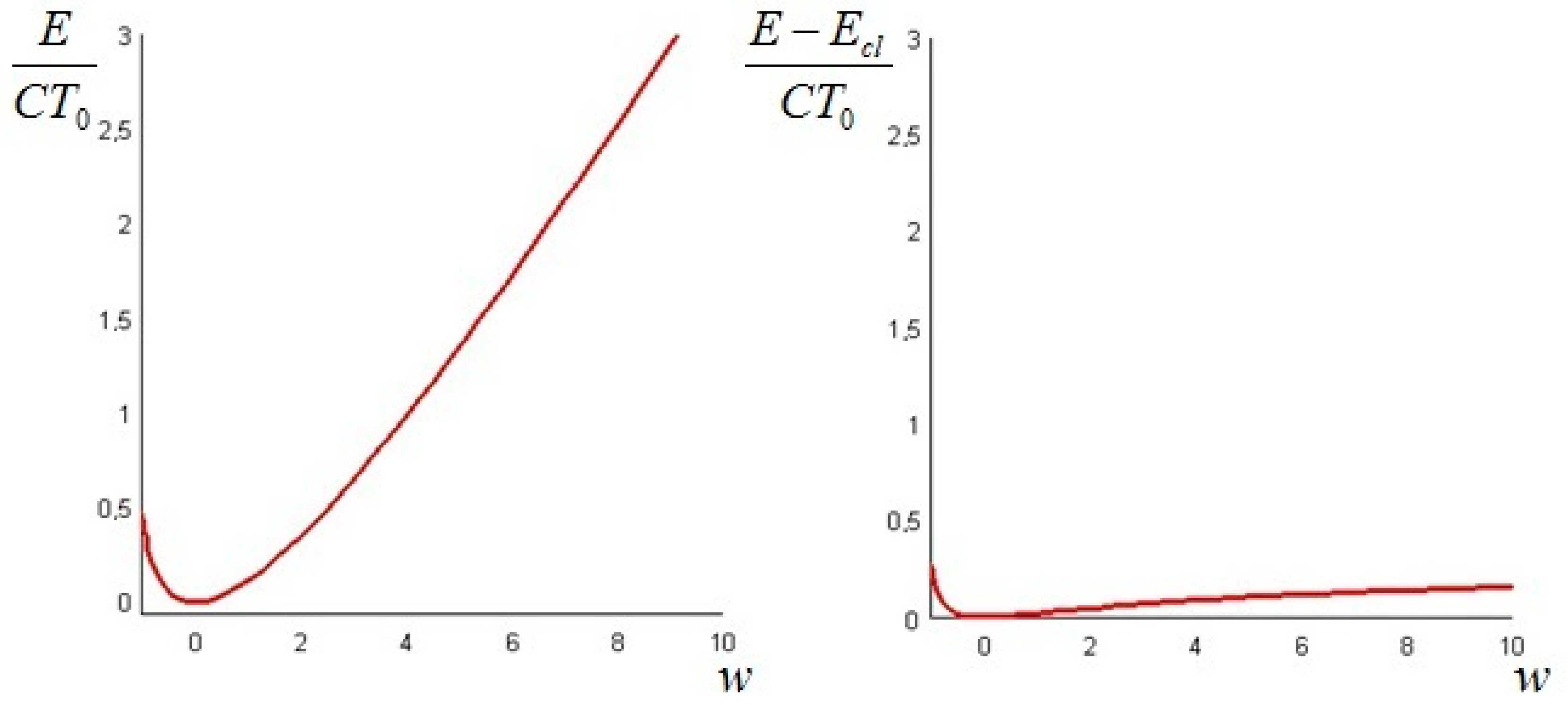
In order to have a positive physical temperature the values of the parameter must be restricted to . The plots of the values of the total exergy of the system, as given by Formula (21), as a function of the parameter (from −4 to 20) and of from Equation (24) are displayed in Figure 1. Both are made dimensionless by dividing them by a “reference energy level” ρcLT0, namely that of the bar at a uniform ambient temperature.
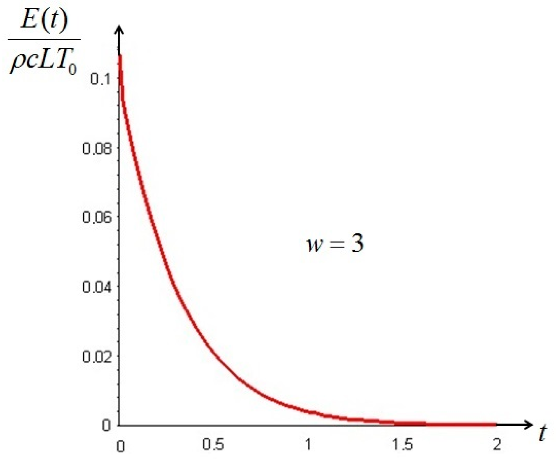
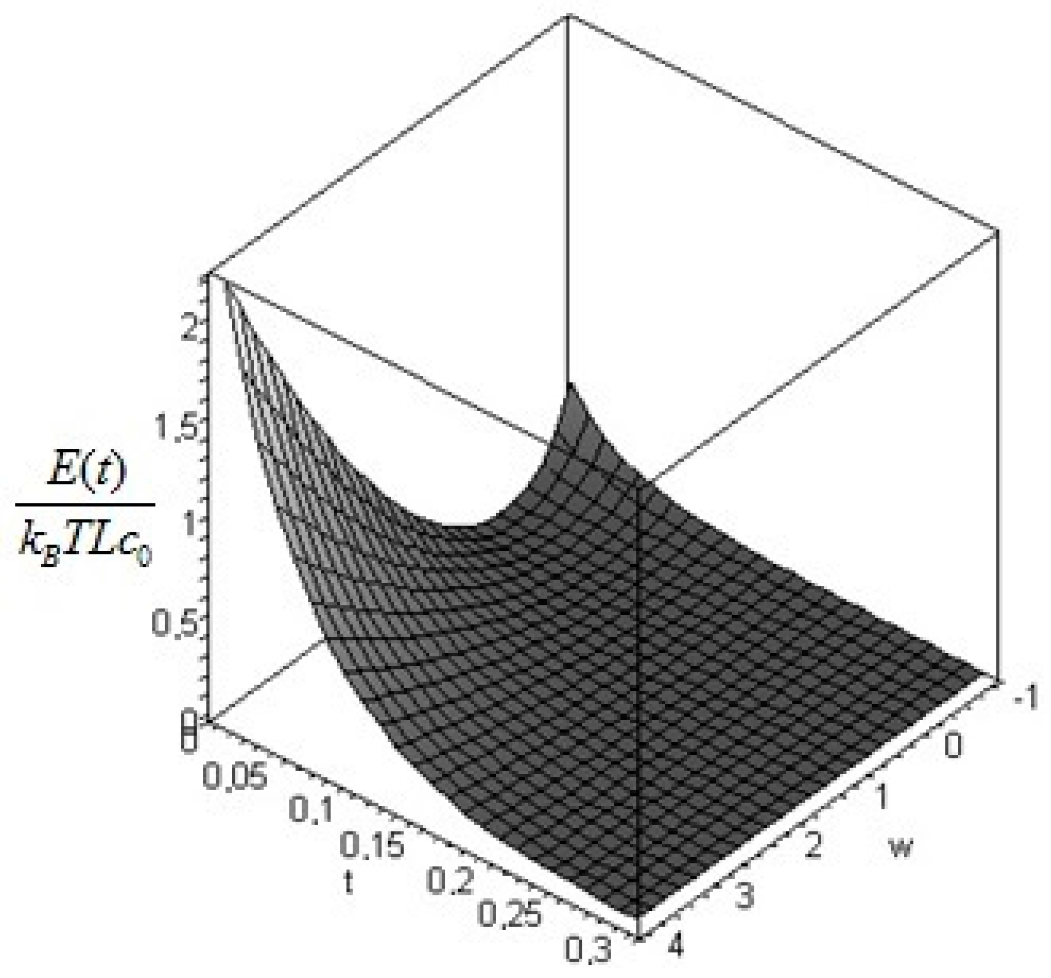
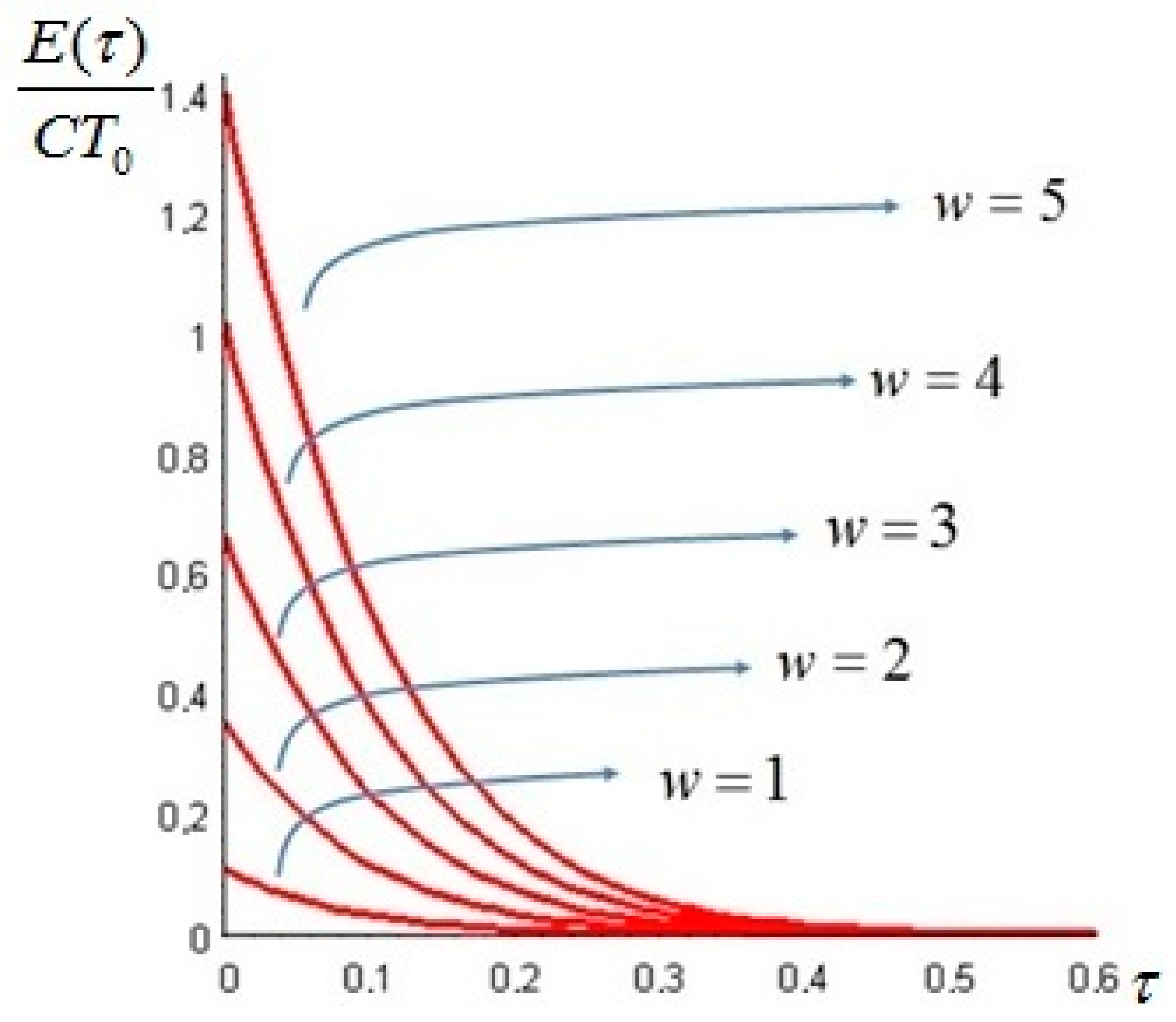
It is interesting to remark that if the initial temperature distribution is—partially or in its entirety—lower than T0 (w < 0), the difference between the non-equilibrium and the classical exergy is of the same order of magnitude as the classical exergy, while at initial temperatures above T0 (w > 0) the difference is of one order lower than the classical exergy: this is in complete agreement with the prescriptions of the Second Law. This result is important, because a vertical segment between the red curve of Figure 1, right, and the axis of the abscissae quantifies the amount of additional work that can be ideally extracted from the system, as shown in Figure 2 for w = 3 and a Biot number equal to 1.
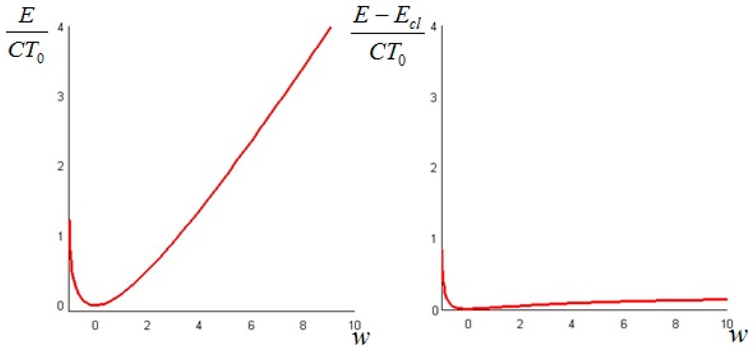
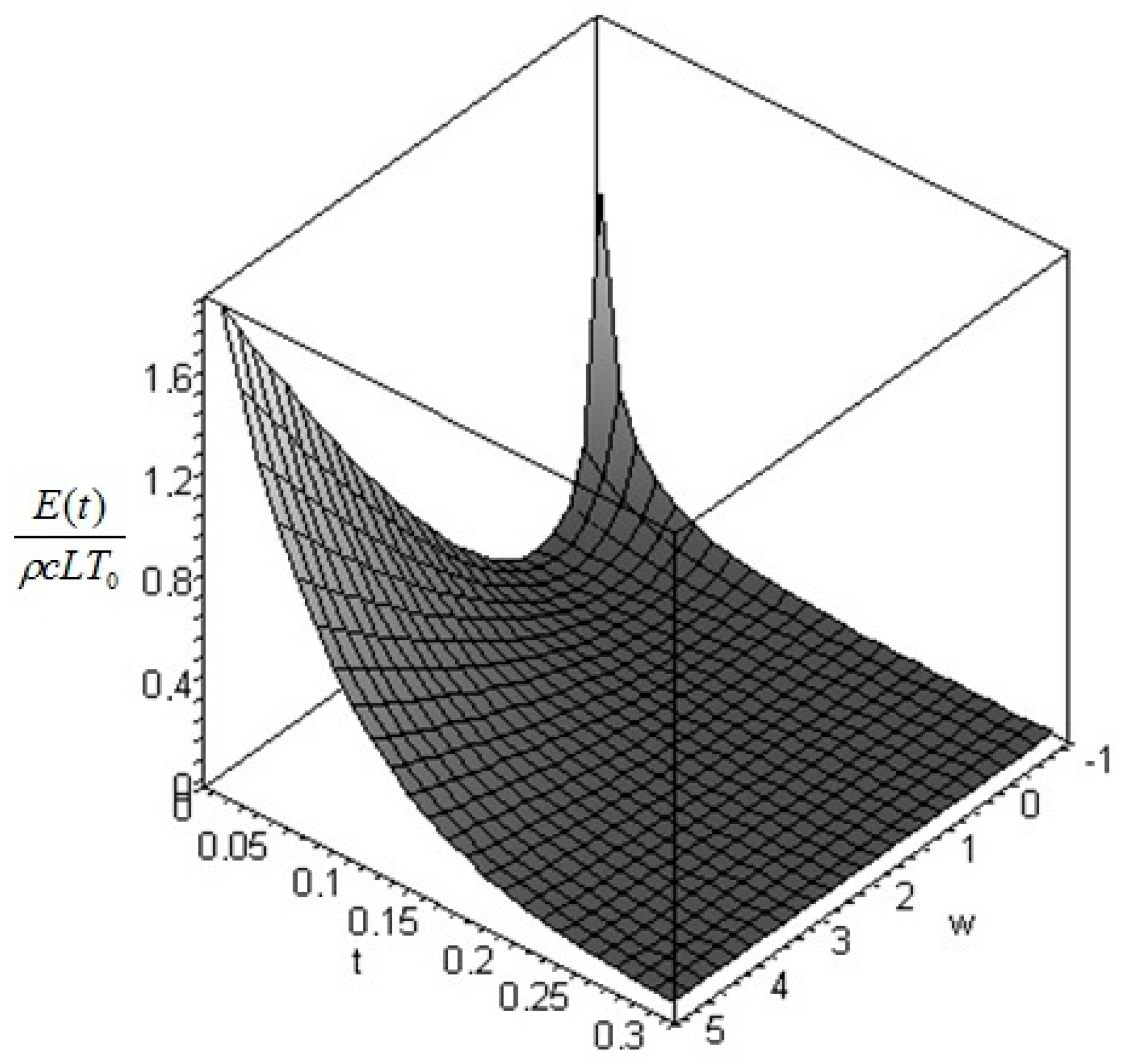
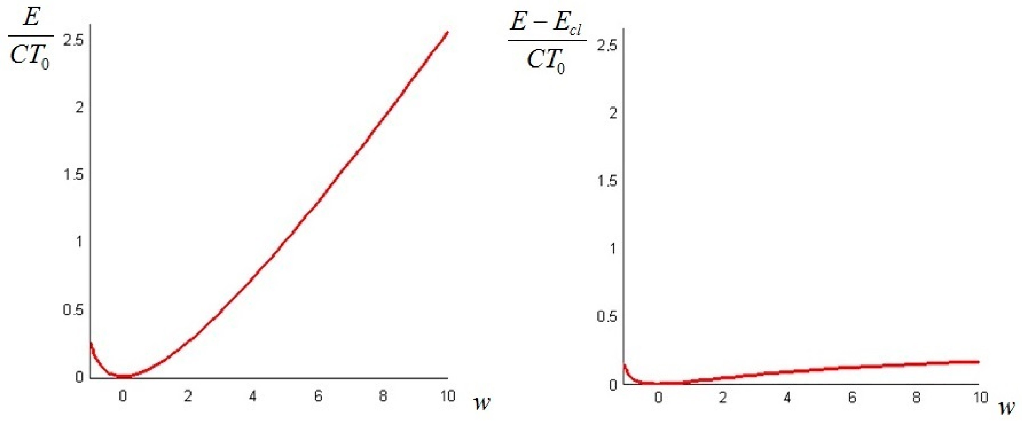
If the initial temperature distribution is given instead by the sum of with its first Fourier mode, that is
where again we can set and rewrite the initial condition as
The physical requirement of a positive definite temperature restricts the acceptable values of the parameter to . The dimensionless plots of the values as a function of (from −1 to 10) and of are given in Figure 3: similar remarks apply as in the previous case.
8.2. A Nanotube with an Initial Uneven Concentration
Let us consider a tube of length L and cross section s2, again with . We assume that there is an initial uneven concentration inside the tube. The initial concentration is given by . The surroundings are at a constant concentration .
To calculate the evolution in time of the concentration we assume that Fick’s law holds. If no material exchange with the surrounding is possible (impermeable boundary conditions), the concentration evolves according to
where is the final equilibrium temperature given by the arithmetic mean over the bar of the initial profile:
where the constants are the Fourier coefficients
If the system boundaries are permeable [31], the concentration evolves according to
where the are the positive roots of .
Suppose the initial concentration is . As before the value of , which is fundamentally a parametric measure of the “amplitude” of the derangement of the initial distribution from the constant one, is constrained to be greater than −1. The total non-equilibrium exergy of the system is given by Equation (34). Figure 5 shows a plot of the total dimensionless non-equilibrium exergy for varying in the range (−1, 10) and of the difference (the difference between the total non-equilibrium exergy and the classical equilibrium exergy) given by Equation (36). Notice that the reference energy is now the Boltzmann concentration energy. It is clear that, for all considered values of w, the deviation of the non-equilibrium chemical exergy from its equilibrium counterpart is of one order of magnitude lower than the latter. A plot of (Equation (33)) is given in Figure 6.
8.3. Non-Equilibrium Exergy of a Pin Fin: A Simple Model
Consider (Figure 7) a pin fin heat sink constituted by a set of cylindrical homogeneous metallic pins of length L and cross section A. Following common practice, the pin exchanges heat with the surroundings at T0 by convection on its lateral surface, while its wall-end is at a constant temperature . If the diameter of the rod is sufficiently smaller than its length and the material thermal conductivity sufficiently high, there will be no radial temperature distribution in the cylinder.
The convection exchange at the surface is assumed to be described by a constant heat transfer coefficient , so that the corresponding equations for the evolution of the temperature are given by
Here, is a constant parameter proportional to the heat transfer coefficient depending on the geometry and on the heat capacity of the pin.
If we define the function corresponding to the steady state ( is the Biot number) and introduce the dimensionless rod length y = x/L:
Notice that the function is bounded between 0 and 1 in the domain [0 ≤ y ≤ 1]. The evolution of the temperature is explicitly described by
where the dimensionless time is given by . The eigenvalues are the roots of the equation , while the Fourier coefficients are given by
and depend on the initial temperature profile .
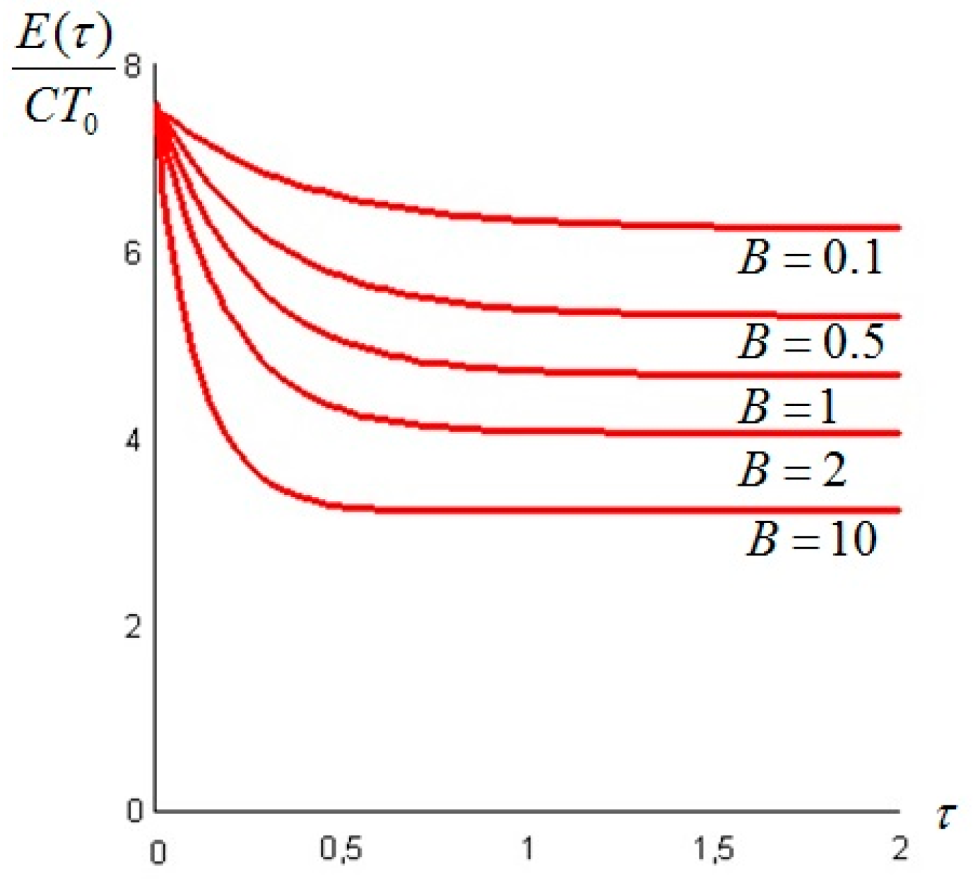
Let us analyze the simple case of an initial linear distribution of temperature, given by
The explicit form of the temperature evolution in this case is
Introducing the dimensionless variables defined by the relation , Equation (50) can be written in dimensionless form:
The exergy of the system at time t is given by Equation (20), and a plot for different values of Bi is presented in Figure 8.
The total exergy is given by the difference between the exergy at time and the exergy at time (Equation (21)): notice that now this quantity may also take negative values, which means that the exergy of the final state is higher than the exergy of the initial state. For example, if the initial temperature distribution is such that a region of the bar between some x and L is initially at a temperature lower than T0, then the final equilibrium distribution can be reached only if the pin absorbs some amount of thermal exergy from the environment: the maximum ideally extractable work increases accordingly.
8.4. A Non-Isothermal Axisymmetric Thin Disc Immersed in a Thermal Bath at T0
We consider a thin disc, with radius R and thickness s, immersed in a thermal bath at . If the surface of the disk is insulated and external thermal exchange can take place only around the surface 2πRs, then the temperature evolves according to
where and are the roots of the Bessel function , that is . The coefficients are given by
and the equilibrium temperature by
If we allow for a thermal exchange with the surroundings, the temperature evolves according to
where now
and the constants are the roots of , where Bi is the Biot number of the system and the values are defined by .
If we assume that the initial profile is a constant, say , then, from Equation (22) we obtain
where is the heat capacity of the disk.
Next, let us examine an initial condition corresponding to a bell-shaped temperature distribution (increasing toward the center of the disk):
The temperature at the center of the disk is controlled by , since at r = 0 the temperature is and then it rises (or decreases) to the environment temperature . Again the constraint is applies. From Equation (22) we obtain:
giving
The difference between the non-equilibrium exergy and its classical counterpart is explicitly calculated as
Plots of the total dimensionless non-equilibrium exergy and of for −1 < w < 10 are given in Figure 9.
8.5. A Sphere with an Initial Uneven Temperature Distribution Immersed in a Homogeneous Environment at T0
In this section, we consider a homogeneous sphere with a radius R immersed in a thermal bath at . For the sake of simplicity, the initial condition is assumed to depend only on . If the surface of the sphere is insulated, then the temperature evolves according to
where and are the roots of . The coefficients are given by
and is the equilibrium temperature given by
where the integral in dV must be performed over the volume of the sphere.
If we allow for a thermal exchange with the surroundings, the temperature evolves according to
where and are the roots of and is the Biot number of the system. The coefficients are now given by
If we assume that the initial profile is a constant, say , then
Let us examine though a more interesting situation one for which the initial condition corresponds to a bell-shaped radial temperature distribution. In analogy with the case of the disk, we may take the same type of function (see Equation (58)):
The exergy Equation (22) provides
Thus,
The difference between the non-equilibrium exergy and the classical exergy, given by Formula (23) is calculated as
9. Conclusions
Starting from a system in thermal or concentration non-equilibrium, the evolution of the thermal or concentration fields, respectively, is obtained by analytically solving the applicable diffusion equation. Three quantities are of interest in the present context (x denotes here the proper coordinate vector):
- (1)
- The Gibbs’ available energy A(t = 0), defined as the double integral (in space and time) of the quantity from x = 0 to x = X and from t = 0 to t = ∞, when the system has reached its adiabatic internal equilibrium at Teq;
- (2)
- The classical equilibrium exergy E(t = 0), defined as the double integral (in space and time) of the quantity from x = 0 to x = X and from t = 0 to t = ∞; and
- (3)
- The quantity we call non-equilibrium exergy En-eq(t = 0), defined as the double integral (in space and time) of the quantity from x = 0 to x = X and from t = 0 to t = ∞.
The above quantities attain different values, and while the Gibbs available energy can be directly calculated on the basis of an adiabatic energy balance (to compute the Teq), both the standard and the non-equilibrium exergy require the additional specification of a proper set of boundary conditions. The non-equilibrium exergy is always higher than its equilibrium counterpart, because it contains the portion of extra ideal work that may be extracted from the system in the course of its internal equilibration. No general relation can be derived between the two latter quantities, because the temperature (or concentration) history depend on the imposed boundary conditions and there is no a priori reason for the system to pass through its internal equilibrium state before reaching the final dead state.
Incidentally, since the initial energy level U(0,x) is known and the non-equilibrium exergy E(t,x) has been calculated, a non-equilibrium entropy can be defined for any system as , its value depending on the initial T (or c) profile. Correspondingly, for each initial temperature or concentration distribution—and for a given set of boundary conditions—the initial entropy of the non-equilibrium system is . The original Gibbs entropy/energy plane may be thus extended into a 3-D representation, in which each point in the “non-equilibrium” zone (that obviously corresponds in our model to a different temperature or concentration distribution) is identified by a different non-equilibrium exergy value: this topic is worthy of further investigation, and is the subject of a separate paper [29].
As a final remark, it is important to recall that the use of the Fourier thermal diffusion law for non-equilibrium situations has been—and rightly so—criticized from a phenomenological point of view, because it implies an infinite “transport velocity” for the temperature signal. In systems with gross initial thermal inhomogeneities—however small the subdomains in which the solid is subdivided—the real non-infinite temperature diffusion velocity may bear a strong influence on the results discussed in the previous sections. If the Cattaneo transport law is used, the mathematics become slightly more involved, and at least for some of the examples discussed in this paper, analytical solutions can be found: this subject, too, will be discussed in a separate paper.
Author Contributions
Enrico Sciubba and Federico Zullo contributed equally to this work. All authors have read and approved the final version of the manuscript.
Conflicts of Interest
The authors declare no conflict of interest.
References
- Demirel, Y. Nonequilibrium thermodynamics modeling of coupled biochemical cycles in living cells. J. Non-Newton. Fluid Mech. 2010, 165, 953–972. [Google Scholar] [CrossRef]
- Kleidon, A. A basic introduction to the thermodynamics of the Earth. Philos. Trans. R. Soc. B 2010, 365, 1303–1315. [Google Scholar] [CrossRef] [PubMed]
- Fath, B.D.; Jørgensen, S.E.; Patten, B.C.; Straškraba, M. Ecosystems growth and development. Ecosystems 2004, 77, 213–228. [Google Scholar] [CrossRef] [PubMed]
- Grmela, M.; Grazzini, G.; Lucia, U.; Yahia, L.H. Multiscale Mesoscopic Entropy of Driven Macroscopic Systems. Entropy 2013, 15, 5053–5064. [Google Scholar] [CrossRef]
- Grubbström, R. An attempt to introduce dynamics into generalized exergy considerations. Appl. Energy 2007, 84, 701–718. [Google Scholar] [CrossRef]
- Grubbström, R. On the Exergy Content of an Isolated Body in Thermodynamic Disequilibrium. Int. J. Energy Optim. Eng. 2012, 1, 1–18. [Google Scholar] [CrossRef]
- Jörgensen, S.E. Evolution and exergy. Ecol. Model. 2007, 203, 490–494. [Google Scholar] [CrossRef]
- Jörgensen, S.E.; Fath, B.D. Fundamentals of Ecological Modelling; Elsevier: Amsterdam, The Netherlands, 2001. [Google Scholar]
- Wall, G. Exergy–A Useful Concept within Resource Accounting; Report 77-42; Institute of Theoretical Physics, Chalmers University of Technology and University of Göteborg: Göteborg, Sweden, 1977. [Google Scholar]
- Badescu, V. Optimal paths for minimizing lost available work during usual finite-time heat transfer processes. J. Non-Equilib. Thermodyn. 2004, 29, 53–73. [Google Scholar] [CrossRef]
- Bejan, A. Entropy generation minimization: The new thermodynamics of finite-size devices and finite-time processes. J. Appl. Phys. 1996, 79, 1191–1218. [Google Scholar] [CrossRef]
- Pavelka, M.; Klika, V.; Vagner, P.; Marsk, F. Generalization of exergy analysis. Appl. Energy 2015, 137, 158–172. [Google Scholar] [CrossRef]
- Vagner, P.; Pavelka, M.; Marsk, F. Pitfalls of exergy analysis. J. Non-Equilib. Thermodyn. 2017, 42. [Google Scholar] [CrossRef]
- Hoffmann, K.H.; Andresen, B.; Salamon, P. Measures of dissipation. Phys. Rev. A 1989, 39, 3618–3621. [Google Scholar] [CrossRef]
- Lebon, G.; Jou, D.; Casas-Vazquez, J. Understanding Non-Equilibrium Thermodynamics; Springer: Berlin, Germany, 2008. [Google Scholar]
- Gyarmati, I. Non-Equilibrium Thermodynamics; Springer: Berlin, Germany, 1970. [Google Scholar]
- Prigogine, I. Introduction to Thermodynamics of Irreversible Processes; Interscience Pub: New York, NY, USA, 1955. [Google Scholar]
- Sancho, P.; Llebot, J.E. Thermodynamic entropy and turbulence. Phys. A Stat. Mech. Appl. 1994, 205, 623–633. [Google Scholar] [CrossRef]
- Kotas, T. Teaching the exergy methods to engineers. In Teaching Thermodynamics; Levins, J., Ed.; Springer: New York, NY, USA, 1985; pp. 373–385. [Google Scholar]
- Gibbs, J.W. On the Equilibrium of Heterogeneous Substances, 1875. In The Scientific Papers of J.W. Gibbs; Dover Publications: New York, NY, USA, 1961. [Google Scholar]
- Gaggioli, R.A.; Richardson, D.H.; Bowman, A.J. Available Energy—Part I: Gibbs revisited. J. Energy Resour. Technol. 2002, 124, 105–109. [Google Scholar] [CrossRef]
- Gaggioli, R.; Paulus, D. Available Energy—Part II: Gibbs extended. J. Energy Resour. Technol. 2002, 124, 110–115. [Google Scholar] [CrossRef]
- Hatsopoulos, G.N.; Gyftopoulos, E.P. A Unified Quantum Theory of Mechanics and Thermodynamics. Part I: Postulates. Found. Phys. 1976, 6, 15–31. [Google Scholar] [CrossRef]
- Hatsopoulos, G.N.; Gyftopoulos, E.P. A Unified Quantum Theory of Mechanics and Thermodynamics. Part IIa: Available Energy. Found. Phys. 1976, 6, 127–141. [Google Scholar] [CrossRef]
- Hatsopoulos, G.N.; Gyftopoulos, E.P. A Unified Quantum Theory of Mechanics and Thermodynamics. Part IIb: Stable Equilibrium States. Found. Phys. 1976, 6, 439–455. [Google Scholar] [CrossRef]
- Gyftopolous, E.P.; Beretta, G.P. Thermodynamics: Foundations and Applications; Macmillan Pub: London, UK, 1991. [Google Scholar]
- Gaggioli, R.A. Teaching elementary thermodynamics and energy conversion: Opinions. Energy 2010, 35, 1047–1056. [Google Scholar] [CrossRef]
- Gaggioli, R.A. The dead state. Int. J. Thermodyn. 2012, 15, 191–199. [Google Scholar] [CrossRef]
- Sciubba, E.; Zullo, F. A novel derivation of the time evolution of the entropy of non-equilibrium macroscopic systems. Entropy 2017, in press. [Google Scholar]
- Zullo, F. Entropy Production in the Theory of Heat Conduction in Solids. Entropy 2016, 18, 87. [Google Scholar] [CrossRef]
- Parti, M. Mass transfer Biot numbers. Period. Polytech. Eng. Mech. Eng. 1994, 38, 109–122. [Google Scholar]
Figure 1.
Total exergy of the bar (left); and difference between the non-equilibrium and the classical exergy (right), as a function of w = T1/T0.
Figure 1.
Total exergy of the bar (left); and difference between the non-equilibrium and the classical exergy (right), as a function of w = T1/T0.

Figure 2.
Time decay of the non-equilibrium exergy of the bar .

Figure 3.
Plots of the total exergy (left); and of the difference between the non-equilibrium and the classical exergy (right), for the initial condition (Equation (39)) and as a function of = T1/T0.
Figure 3.
Plots of the total exergy (left); and of the difference between the non-equilibrium and the classical exergy (right), for the initial condition (Equation (39)) and as a function of = T1/T0.

Figure 4.
Profile of the dimensionless exergy of the bar as a function of time and of = T1/T0 for the initial profile (Equation (41)).
Figure 4.
Profile of the dimensionless exergy of the bar as a function of time and of = T1/T0 for the initial profile (Equation (41)).

Figure 5.
The total exergy of the nanotube (left); and the difference between the non-equilibrium and the classical exergy (right) as a function of w.
Figure 5.
The total exergy of the nanotube (left); and the difference between the non-equilibrium and the classical exergy (right) as a function of w.

Figure 6.
The profile of the exergy of the nanotube as a function of time and of for the initial profile .
Figure 6.
The profile of the exergy of the nanotube as a function of time and of for the initial profile .

Figure 7.
(left) A slender pin-fin arrangement; (right) the model pin analyzed.

Figure 8.
A dimensionless plot of the exergy of the system as given by Equation (20), for , , and Bi as a parameter.
Figure 8.
A dimensionless plot of the exergy of the system as given by Equation (20), for , , and Bi as a parameter.

Figure 9.
The total exergy of the disc (left); and the difference between the non-equilibrium and the classical exergy (right) for the initial profile given by Equation (58) as a function of w = T1/T0.
Figure 9.
The total exergy of the disc (left); and the difference between the non-equilibrium and the classical exergy (right) for the initial profile given by Equation (58) as a function of w = T1/T0.

Figure 10.
The total exergy of the sphere (left); and the difference between the non-equilibrium and the classical exergy (right) for the initial profile (Equation (68)).
Figure 10.
The total exergy of the sphere (left); and the difference between the non-equilibrium and the classical exergy (right) for the initial profile (Equation (68)).

Figure 11.
Time evolution of the exergy of the sphere from the initial profile given by Equation (68) for different values of the parameter = T1/T0.
Figure 11.
Time evolution of the exergy of the sphere from the initial profile given by Equation (68) for different values of the parameter = T1/T0.

© 2017 by the authors. Licensee MDPI, Basel, Switzerland. This article is an open access article distributed under the terms and conditions of the Creative Commons Attribution (CC BY) license (http://creativecommons.org/licenses/by/4.0/).
Share and Cite
MDPI and ACS Style
Sciubba, E.; Zullo, F. Exergy Dynamics of Systems in Thermal or Concentration Non-Equilibrium. Entropy 2017, 19, 263. https://doi.org/10.3390/e19060263
AMA Style
Sciubba E, Zullo F. Exergy Dynamics of Systems in Thermal or Concentration Non-Equilibrium. Entropy. 2017; 19(6):263. https://doi.org/10.3390/e19060263
Chicago/Turabian StyleSciubba, Enrico, and Federico Zullo. 2017. "Exergy Dynamics of Systems in Thermal or Concentration Non-Equilibrium" Entropy 19, no. 6: 263. https://doi.org/10.3390/e19060263
Note that from the first issue of 2016, this journal uses article numbers instead of page numbers. See further details here.