Combining Faraday Tomography and Wavelet Analysis
by
 , and
, and
Dmitry Sokoloff
1,2,*, 
Rainer Beck
3, 
Anton Chupin
4,5,
Peter Frick
4,6,
George Heald
7 and
Rodion Stepanov
4 1
Department of Physics, Moscow University, 119992 Moscow, Russia
2
Institute of Terrestrial Magnetism, Ionosphere and Radio Wave Propagation, Kaluzhskoe Hwy 4, Troitsk, 108840 Moscow, Russia
3
MPI für Radioastronomie, Auf dem Hügel 69, 53121 Bonn, Germany
4
Institute of Continuous Media Mechanics, Korolyov str. 1, 614061 Perm, Russia
5
Department of Mechanics and Mathematics, Perm State National Research University, Bukirev str. 15, 614990 Perm, Russia
6
Department of General Physics, Perm State National Research University, Bukirev str. 15, 614990 Perm, Russia
7
CSIRO Astronomy and Space Science, P.O. Box 1130, Bentley, WA 6102, Australia
*
Author to whom correspondence should be addressed.
Galaxies 2018, 6(4), 121; https://doi.org/10.3390/galaxies6040121
Submission received: 3 October 2018
/
Revised: 16 November 2018
/
Accepted: 19 November 2018
/
Published: 22 November 2018
(This article belongs to the Special Issue The Power of Faraday Tomography)
Abstract
:We present a concept for using long-wavelength broadband radio continuum observations of spiral galaxies to isolate magnetic structures that were only previously accessible from short-wavelength observations. The approach is based on combining the RM Synthesis technique with the 2D continuous wavelet transform. Wavelet analysis helps to isolate and recognize small-scale structures which are produced by Faraday dispersion. We find that these structures can trace galactic magnetic arms as illustrated by the case of the galaxy NGC 6946 observed at cm. We support this interpretation through the analysis of a synthetic observation obtained using a realistic model of a galactic magnetic field.
1. Introduction
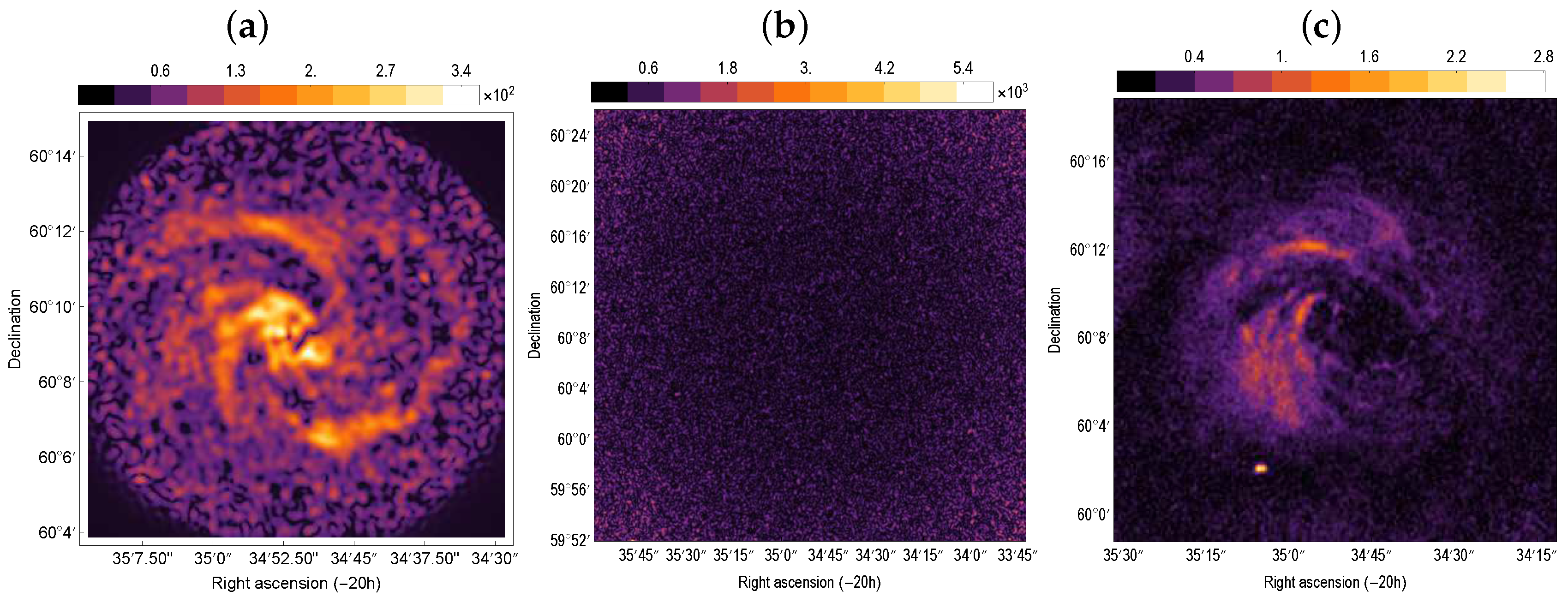
The bulk of contemporary knowledge concerning magnetic field configurations in spiral galaxies has been obtained using observations performed at only a few wavelengths. Modern progress in observational techniques allows us to observe galaxies at dozens to hundreds or even thousands of individual wavelengths over broad bands. However, it is important to learn how best to use these new resources. Some problems which can arise are illustrated in Figure 1. The left panel shows the linearly polarized intensity distribution of NGC 6946 at cm with a bandwidth of 100 MHz from Beck et al. [1]. Magnetic spiral arms are clearly recognized. Magnetic arms are important because they are possibly the sign of magnetic reconnection regions [2] or may also be products of dynamo action [3]. However their origin remains unclear [4]. The middle panel shows the polarized intensity distribution obtained using a single narrowband frequency channel around cm from modern broadband observations in the spectral range from 17 to 22 cm. The plot shows only noise. The discrepancy occurs for two reasons. First, sensitivity in modern radio continuum observations is built up through a combination of time and bandwidth, so narrowband images have relatively high noise. Second, depolarization effects by Faraday rotation are much more pronounced at longer wavelengths as compared to cm.
One can try resolve the problem in two ways. Firstly, it is possible to sum polarized intensities over all channels in the range cm to emulate single-wavelength observations at cm. This option is not optimal because it does not fully exploit the possibilities offered by modern observational techniques. Another option is to use RM Synthesis [5,6] which involves coherently adding data at many wavelengths for many values of Faraday depth. RM Synthesis is a technique giving a “Faraday cube” which consists of the “Faraday dispersion function” F (also called “Faraday spectrum”) for each pixel on the sky plane
where is the Faraday depth, P is the complex polarization, and are the sky coordinates of the pixel, and and define the range of observed wavelengths. Reconstruction of the magnetic field even along a single line of sight remains a challenging problem [7]. Three-dimensional Faraday spectrum data (i.e., the distribution of polarized intensity as a function of Faraday depth) can be analysed in various ways. A straightforward approach is to compute maximum intensity values [8] (the peak polarized intensity ). The resulting distribution of is shown in Figure 1c. The recovered signal-to-noise is much higher than in Figure 1b. However, we still do not see as prominently the narrow magnetic arms visible in Figure 1a because they are suppressed by Faraday depolarization effects at cm.
We face a difficult choice: to postpone broadband observations of magnetic arms in spiral galaxies until the forthcoming SKA telescope will be ready for observations with its substantially higher sensitivity, or to develop a method which allows recovery of magnetic arms from the available broadband data taken at long wavelengths. The second way seems more attractive. The suggested method is fully described by Chupin et al. [9]. In the present paper, we summarize the idea and illustrate it by a comparison of wavelet transform of the NGC 6946 data at cm and at cm (Section 2). We support our interpretation of the method through analysis of an artificial example (Section 3).
2. Idea of the Method Applied to the NGC 6946 Data
We begin by recognizing that polarized observations performed at the wavelength are most informative for magnetic structures of the scale for which is comparable with . Contributions from structures with are strongly depolarized due to Faraday rotation while Faraday rotation from the structures with is too weak to be easily recognized and interpreted. It means that using observations at cm instead of at cm we deal with magnetic structures that are an order of magnitude smaller (). In other words, instead of detecting magnetic arms by observing polarized emission on large scales directly, we instead seek small-scale structures which can arise by tangling and randomizing of large-scale structures, in addition to small-scale structures which arise from the small-scale turbulent magnetic fields that are predicted by dynamo theory.
In practice, the realization of the idea suggested in [9] is based on the wavelet technique. Wavelet functions are used for the analysis of spatial and temporal data, also in astrophysics [10]. The wavelet transform can be used as an enhancement of RM Synthesis to analyze structure at different scales [11,12]. Here wavelets are used as a spatial-scale filtering tool. We decompose the two-dimensional map into wavelet coefficients of various scales l:
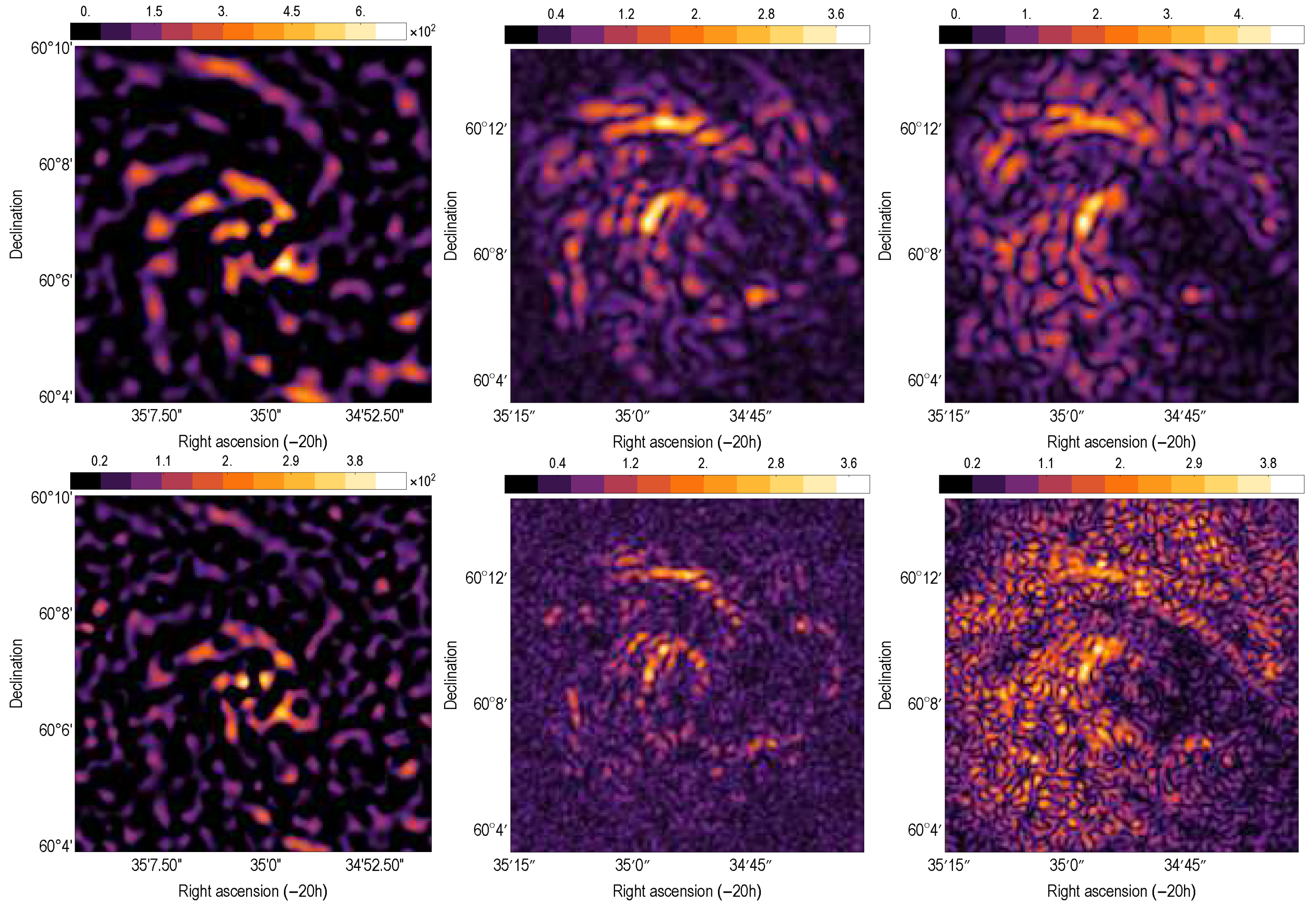
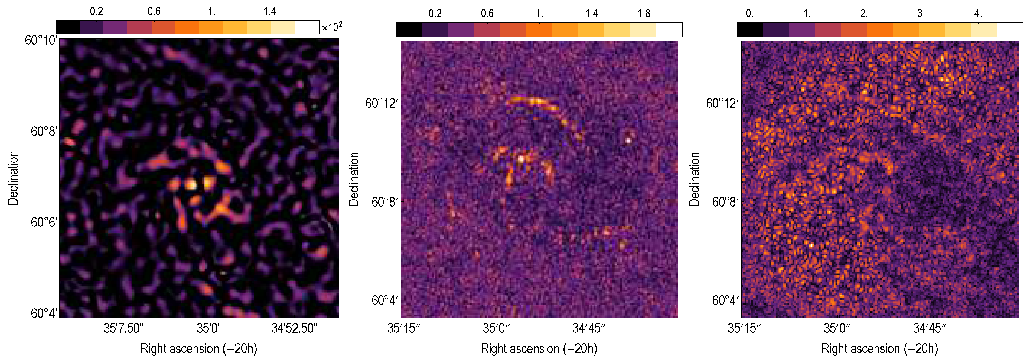
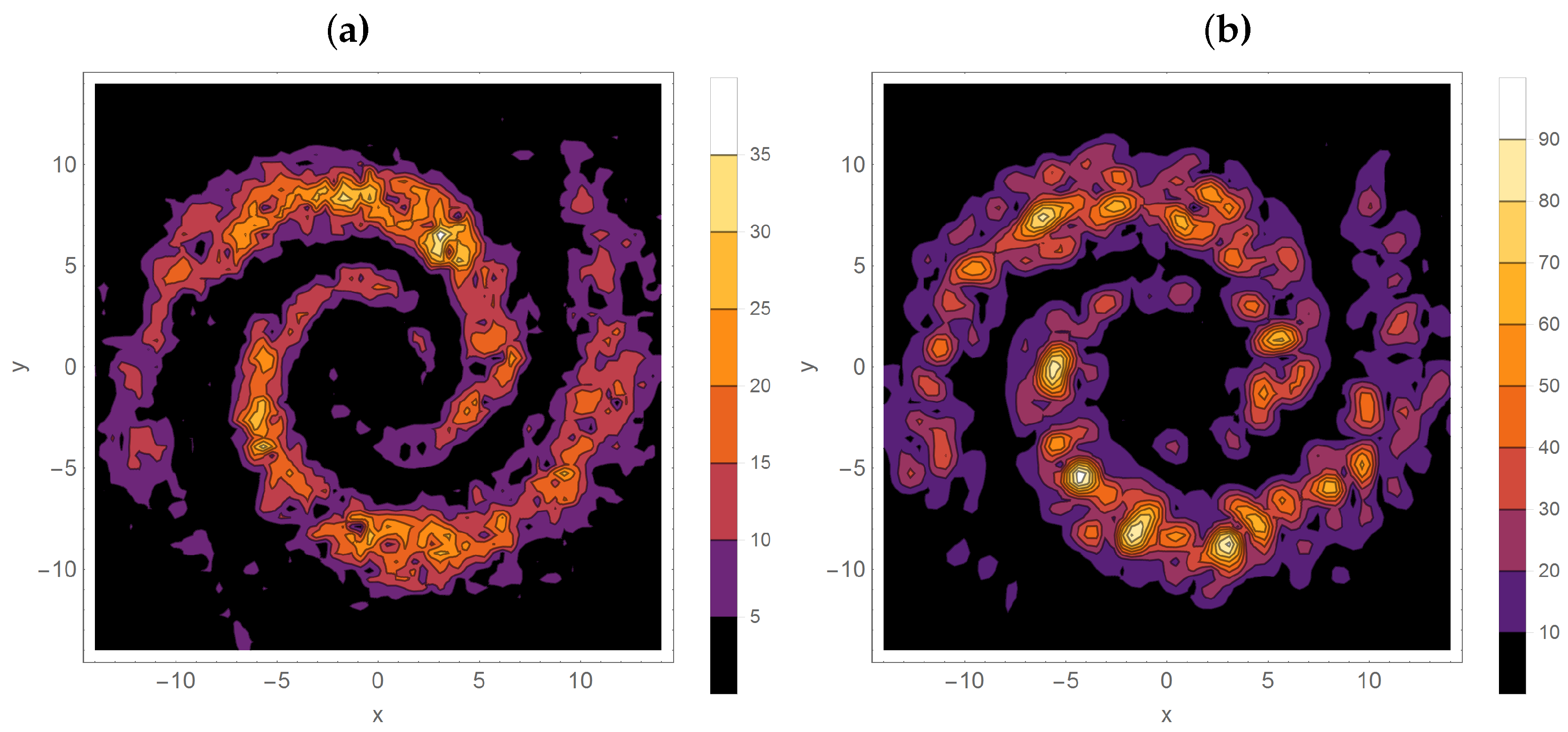
using the “Mexican-hat” wavelet as the base wavelet and scale a as the characteristic radius of the wavelet function. For the wavelet transform one can define a peak intensity distribution along each line of sight. Results for various scales l measured in arcseconds are shown in the middle column of Figure 2. We recognize small-scale structures at the scale (middle row) arcsec that are organized into arm-like structures. Structures at smaller (lower row) and larger (upper row) scales are less pronounced. In other words, we have thus traced the structure of magnetic arms known from cm using data obtained at cm despite the lack of a direct detection of large-scale arm-like structure. In a comparison, the result of wavelet decomposition of polarized intensity at 6 cm (left column of Figure 2) and of the peak Faraday spectra (right column of Figure 2) are much noisier. These images repeat similar results from [9] except for 6 cm, which was calculated and added to the panel to aid comparison.
3. Synthetic Data Analysis
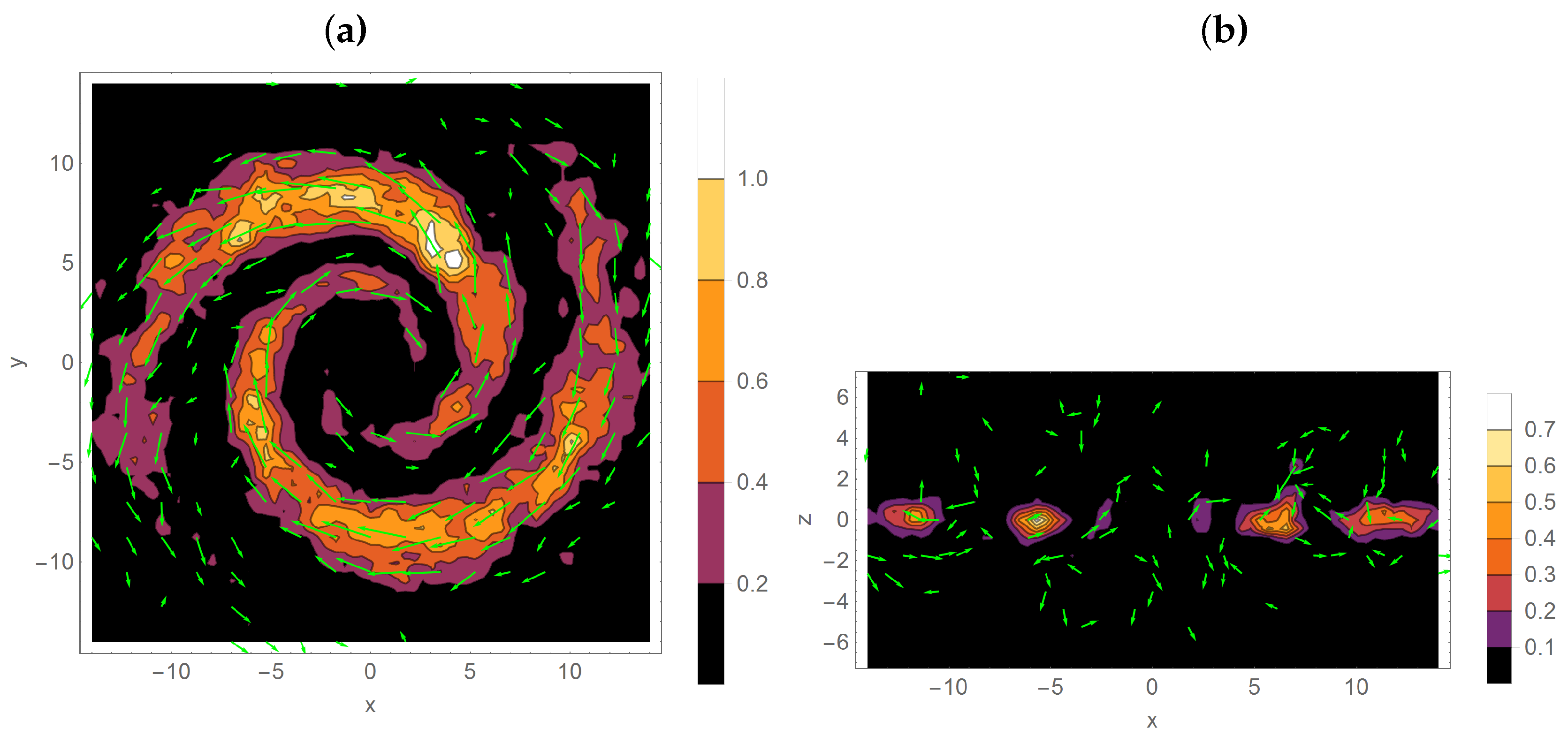
We now consider a model magnetic field in order to demonstrate qualitatively the applicability of our approach and to support our interpretation of the observational results. The galactic magnetic field is modelled as a superposition of a large-scale component and a small-scale turbulent component :
where is the position vector in the cylindrical coordinate system (. The regular part of the magnetic field is assumed to be of bisymmetric form with two reversals along azimuthal angle:
where is the field amplitude (strength) and is the azimuthal phase of the mode m, p is a pitch angle, and and are the Gaussian radius and vertical scales of the magnetic galactic disk. The tanh term is introduced to suppress the field near the centre of the galaxy and thus to avoid a discontinuity near the axis [13]. The components of the regular magnetic field are then evaluated by
with the relation (7) being a result of the incompressibility condition.
The turbulent magnetic field is considered as a divergence-free, random fluctuating field with the energy spectrum given by , and a Gaussian spatial distribution with characteristic radius and vertical scale :
where is the strength of the turbulent field. The spectral properties of the random function are specified as follows:
We adopt (Kolmogorov scaling), , and [14].
Figure 3 shows the distribution of galactic magnetic field in the three-dimensional numerical domain with resolution for a particular choice of parameters: , , , , , , and . Thermal electron and cosmic rays densities are adjusted to obtain qualitative correspondence with the observations considered earlier. We use this simulated magnetic field to calculate artificial maps of polarized intensity and Fadaray rotation for discrete values of in the observed range from 17 to 22 cm. Then a synthetic RM-cube is analysed through the same approach as for the observed NGC 6946 data in Section 2.
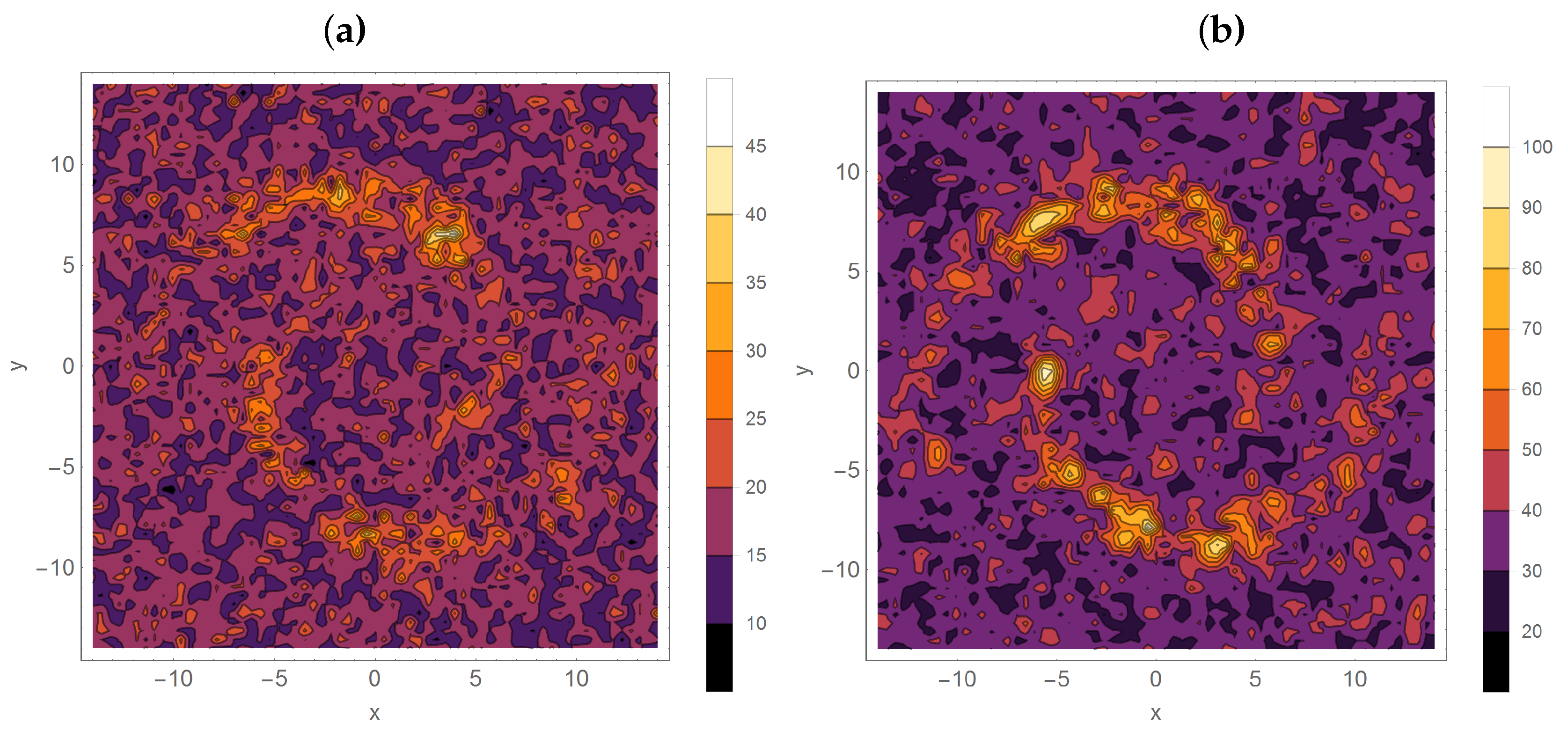
For the case of a noise-free observation of the polarized intensity, the distribution of (which is shown in Figure 4a) is slightly affected by Faraday depolarization. We note that the result does not differ from the initial distribution in Figure 3a because the rotation measures are rather moderate (a few tens of rad/m) and the beam depolarization effect is not taken into account. However, the synchrotron emission is considerably scattered over a range of Faraday depths so that small-scale structures appear in the distribution of (see Figure 4b). Nevertheless the large-scale structure of galactic magnetic arm is well traced by .
The situation is substantially changed in the case where white noise is added to the ideal observations such that . Figure 5 shows the resulting distribution of and in the presence of this mock observational noise. The galactic signal in representation is getting much weaker. At the same time the distribution of reveals the magnetic arms with a patchy structure.
4. Discussion
In this paper, we exploit a method [9] that allows us to use long-wavelength broadband observations to isolate magnetic structures that were only previously accessible from short-wavelength observations. The difference between the wavelet analysis of broadband and single-frequency observations is illustrated in the case of NGC 6946. Our interpretation of the method is that we isolate small-scale structures in the RM-cube which are associated with an initially large-scale magnetic field structure that has been distorted by Faraday dispersion. We support this interpretation through the analysis of a synthetic observation generated using a realistic model of a galactic magnetic field with regular and random components. The results presented here demonstrate that the method can be helpful in practice especially in the case of polarization data with low signal-to-noise at individual wavelengths. However, we point out that intrinsically small-scale structures of the magnetic field may contribute to the wavelet coefficients. The existence of such structures has been a general expectation from dynamo theory, but the previous methods do not allow us to isolate this. We note that the wavelet technique can be successfully combined with modern approaches like Faraday tomography [15] and the method based on synchrotron polarization gradients [16]. The assessment of an anisotropic structure of the galactic magnetic can be done using anisotropic wavelets [17,18]. With these approaches, one can probe the local interstellar medium in the Galactic foreground towards some galaxies [19]. Our model of a realistic galactic magnetic field may be also useful for consistent validation of different processing techniques.
Author Contributions
The idea of the method presented here belongs to R.S. and A.C., P.F. embedded the method in the general framework of wavelet methods, D.S. is responsible for the link with dynamo studies, R.B. elaborated the link with classical RM-synthesis, the observational data exploited was obtained by G.H.
Funding
This research was supported by [Russian Foundation for Basic Research], grant number [18-02-00085]; and [Russian Science Foundation], grant numbers [16-41-02012] and [18-1-1-77-1].
Acknowledgments
Numerical simulations were performed on the supercomputers URAN and TRITON of Russian Academy of Science, Ural Branch.
Conflicts of Interest
The authors declare no conflict of interest.
Abbreviations
The following abbreviations are used in this manuscript:
| NGC | New General Catalogue |
| SKA | Square Kilometre Array |
| RM | Rotation measure |
References
- Beck, R.; Frick, P.; Stepanov, R.; Sokoloff, D. Recognizing magnetic structures by present and future radio telescopes with Faraday rotation measure synthesis. Astron. Astrophys. 2012, 543, A113. [Google Scholar] [CrossRef] [Green Version]
- Weżgowiec, M.; Ehle, M.; Beck, R. Hot gas and magnetic arms of NGC 6946: Indications for reconnection heating? Astron. Astrophys. 2016, 585, A3. [Google Scholar] [CrossRef]
- Beck, R. Magnetic fields in spiral galaxies. Astron. Astrophys. Rev. 2015, 24, 4. [Google Scholar] [CrossRef] [Green Version]
- Chamandy, L.; Shukurov, A.; Subramanian, K. Magnetic spiral arms and galactic outflows. Mon. Not. R. Astron. Soc. 2015, 446, L6–L10. [Google Scholar] [CrossRef]
- Burn, B.J. On the depolarization of discrete radio sources by Faraday dispersion. Mon. Not. R. Astron. Soc. 1966, 133, 67. [Google Scholar] [CrossRef]
- Brentjens, M.A.; de Bruyn, A.G. Faraday rotation measure synthesis. Astron. Astrophys. 2005, 441, 1217–1228. [Google Scholar] [CrossRef] [Green Version]
- Sun, X.H.; Rudnick, L.; Akahori, T.; Anderson, C.S.; Bell, M.R.; Bray, J.D.; Farnes, J.S.; Ideguchi, S.; Kumazaki, K.; O’Brien, T.; et al. Comparison of Algorithms for Determination of Rotation Measure and Faraday Structure. I. 1100–1400 MHz. Astron. J. 2015, 149, 60. [Google Scholar] [CrossRef]
- Heald, G.; Braun, R.; Edmonds, R. The Westerbork SINGS survey. II Polarization, Faraday rotation, and magnetic fields. Astron. Astrophys. 2009, 503, 409–435. [Google Scholar] [CrossRef]
- Chupin, A.; Beck, R.; Frick, P.; Heald, G.; Sokoloff, D.; Stepanov, R. Magnetic arms of NGC6946 traced in the Faraday cubes at low radio frequencies. Astron. Nachr. 2018, 339, 440–446. [Google Scholar] [CrossRef]
- Schwinn, J.; Baugh, C.M.; Jauzac, M.; Bartelmann, M.; Eckert, D. Uncovering substructure with wavelets:proof of concept using Abell 2744. Mon. Not. R. Astron. Soc. 2018, 481, 4300–4310. [Google Scholar] [CrossRef]
- Frick, P.; Sokoloff, D.; Stepanov, R.; Beck, R. Wavelet-based Faraday rotation measure synthesis. Mon. Not. R. Astron. Soc. 2010, 401, L24–L28. [Google Scholar] [CrossRef] [Green Version]
- Frick, P.; Sokoloff, D.; Stepanov, R.; Beck, R. Faraday rotation measure synthesis for magnetic fields of galaxies. Mon. Not. R. Astron. Soc. 2011, 414, 2540–2549. [Google Scholar] [CrossRef] [Green Version]
- Stepanov, R.; Arshakian, T.G.; Beck, R.; Frick, P.; Krause, M. Magnetic field structures of galaxies derived from analysis of Faraday rotation measures, and perspectives for the SKA. Astron. Astrophys. 2008, 480, 45–59. [Google Scholar] [CrossRef] [Green Version]
- Stepanov, R.; Shukurov, A.; Fletcher, A.; Beck, R.; La Porta, L.; Tabatabaei, F. An observational test for correlations between cosmic rays and magnetic fields. Mon. Not. R. Astron. Soc. 2014, 437, 2201–2216. [Google Scholar] [CrossRef]
- Ferrière, K. Faraday tomography: A new, three-dimensional probe of the interstellar magnetic field. J. Phys. Conf. Ser. 2016, 767, 012006. [Google Scholar] [CrossRef]
- Lazarian, A.; Yuen, K.H. Gradients of Synchrotron Polarization: Tracing 3D Distribution of Magnetic Fields. Astrophys. J. 2018, 865, 59. [Google Scholar] [CrossRef]
- Frick, P.; Stepanov, R.; Beck, R.; Sokoloff, D.; Shukurov, A.; Ehle, M.; Lundgren, A. Magnetic and gaseous spiral arms in M83. Astron. Astrophys. 2016, 585, A21. [Google Scholar] [CrossRef]
- Ossenkopf-Okada, V.; Stepanov, R. Measuring the filamentary structure of interstellar clouds through wavelets. arXiv, 2018; arXiv:1811.02082. [Google Scholar]
- Van Eck, C.L.; Haverkorn, M.; Alves, M.I.R.; Beck, R.; de Bruyn, A.G.; Enßlin, T.; Farnes, J.S.; Ferrière, K.; Heald, G.; Horellou, C.; et al. Faraday tomography of the local interstellar medium with LOFAR: Galactic foregrounds towards IC 342. Astron. Astrophys. 2017, 597, A98. [Google Scholar] [CrossRef] [Green Version]
Figure 1.
(a) Polarized intensity distribution in NGC 6946 at , (b) single narrowband channel at cm, and (c) peak Faraday spectra synthesised from cm. All are measured with . Note the different colour scale in each panel.
Figure 1.
(a) Polarized intensity distribution in NGC 6946 at , (b) single narrowband channel at cm, and (c) peak Faraday spectra synthesised from cm. All are measured with . Note the different colour scale in each panel.

Figure 2.
Wavelet coefficient maps at the scales 32, 16 and 8 arcsec (from top to bottom): (left column) at cm, (middle column) , (right column) . All are measured with .
Figure 2.
Wavelet coefficient maps at the scales 32, 16 and 8 arcsec (from top to bottom): (left column) at cm, (middle column) , (right column) . All are measured with .


Figure 3.
Distribution of model magnetic field: (a) in central horizontal galactic plane, (b) in central vertical plane. Colour scale shows magnetic field intensity in . Arrows denote magnetic field direction.
Figure 3.
Distribution of model magnetic field: (a) in central horizontal galactic plane, (b) in central vertical plane. Colour scale shows magnetic field intensity in . Arrows denote magnetic field direction.

Figure 4.
Distributions for a model which consists of large scales and small scales (no noise): (a) , (b) . Colour scale shows values in .
Figure 4.
Distributions for a model which consists of large scales and small scales (no noise): (a) , (b) . Colour scale shows values in .

Figure 5.
Distributions for a model which consists of large scales, small scales and noise: (a) , (b) . Colour scale shows values in .
Figure 5.
Distributions for a model which consists of large scales, small scales and noise: (a) , (b) . Colour scale shows values in .

© 2018 by the authors. Licensee MDPI, Basel, Switzerland. This article is an open access article distributed under the terms and conditions of the Creative Commons Attribution (CC BY) license (http://creativecommons.org/licenses/by/4.0/).
Share and Cite
MDPI and ACS Style
Sokoloff, D.; Beck, R.; Chupin, A.; Frick, P.; Heald, G.; Stepanov, R. Combining Faraday Tomography and Wavelet Analysis. Galaxies 2018, 6, 121. https://doi.org/10.3390/galaxies6040121
AMA Style
Sokoloff D, Beck R, Chupin A, Frick P, Heald G, Stepanov R. Combining Faraday Tomography and Wavelet Analysis. Galaxies. 2018; 6(4):121. https://doi.org/10.3390/galaxies6040121
Chicago/Turabian StyleSokoloff, Dmitry, Rainer Beck, Anton Chupin, Peter Frick, George Heald, and Rodion Stepanov. 2018. "Combining Faraday Tomography and Wavelet Analysis" Galaxies 6, no. 4: 121. https://doi.org/10.3390/galaxies6040121
Note that from the first issue of 2016, this journal uses article numbers instead of page numbers. See further details here.