
Adaptive Nonsingular Fast-Reaching Terminal Sliding Mode Control Based on Observer for Aerial Robots

College of Automation, Nanjing University of Aeronautics and Astronautics, Nanjing 211106, China
*
Author to whom correspondence should be addressed.
Actuators 2024, 13(3), 98; https://doi.org/10.3390/act13030098
Submission received: 5 February 2024
/
Revised: 21 February 2024
/
Accepted: 28 February 2024
/
Published: 29 February 2024
(This article belongs to the Special Issue Fault-Tolerant Control for Unmanned Aerial Vehicles (UAVs))
Abstract
:In this article, an observer-based adaptive non-singular fast-reaching terminal sliding mode control strategy is proposed to tackle the problem of actuator faults and uncertain disturbance in aerial robot systems. Firstly, a model of an aerial robot system is established through dynamic analysis. Next, an adaptive observer, combined with a fast adaptive fault estimation (FAFE) algorithm, is proposed to estimate system states and actuator failure and compensate for faults in a precise and prompt manner. In addition, a non-singular fast terminal sliding surface is defined, taking into account the fast convergence of the tracking errors in order to provide appropriate trajectory tracking results. Since the upper bounds of the disturbances caused by the manipulator of the system in practice are unknown, the control approach may benefit from the addition of an adaptive control strategy that can suppress the influence of uncertain disturbances. The Lyapunov stability theory demonstrates that tracking errors are able to converge stably and quickly. In the end, the contrast experiment is conducted to exhibit the effectiveness of the proposed control strategy. The results demonstrate quicker convergence and improved estimating accuracy.
1. Introduction
With the further development of science and the continuous iteration of related technologies, countries and organizations around the world have successively carried out research on multi-rotor aircraft, further promoting the development of drones. In addition to military unmanned reconnaissance aircraft and unmanned target drones, multi-rotor drones also have various civilian applications, including space surveillance, environmental monitoring, surface crack detection, logistics transportation, and so on [1,2,3,4], while these services are no longer able to completely satisfy people’s requirements. With the aim of improving the ability to interact with the external environment, multi-rotor aircraft equipped with multi-joint manipulators, which can help people complete more complex, dangerous, and sophisticated activities, have attracted more and more attention and research [5,6] in recent years. If an autonomous manipulator is combined with the mobile platform on the ground and in the air as a new type of robot, it will have the flexible characteristics of the robotic arm and the mobile platform at the same time, so that the robotic arm can move autonomously and finally be able to grasp the workpiece in industrial production and assist workers in carrying heavy objects [7,8].
This approach, which combines the powerful operation ability of the robotic arm with the free-movement ability of the mobile robot platform to expand the application range of robot technology, has set off a wave of technological development and has broad application prospects. At present, a novel system consisting of a multi-rotor aircraft and a robotic arm can replace people to complete tasks such as sample information collection, instrument remote control, and industrial equipment maintenance [9]. The combination of the robotic arm and the rotorcraft aims to realize the miniaturization and dexterity of the robotic arm and the multi-function and intelligence of the four-rotor aircraft, which conforms to the current technological development trend [10,11].
While the aerial robot enhances its ability to interact with the environment, the drone will also be internally disturbed by the action of the manipulator’s actuator [12]. For a rotorcraft with a robotic arm, when the robotic arm moves, the center of gravity of the whole system will also be affected. To solve this problem, a new adaptive backstepping sliding mode controller was designed in [13]. In [14], after deriving the full dynamics of unmanned aerial manipulation (UAM), the researchers used the low-dimensional simplified model of the entire system and adaptive backstepping technology to deal with the predicament that the unmanned aerial vehicle (UAV) is independent of the robot manipulator control. Reference [15] provided a sliding mode control for the attitude control of the rotorcraft aerial manipulator. In [16], a fuzzy sliding mode control method was developed to obtain stable control performance and tracking performance. For a UAM under uncertainties and external disturbances, an adaptive sliding mode observer-based control strategy was proposed in [17] to achieve the desired steady-state and transient performance.
As a result of a diversity of environments and attitudes, the aircraft will face various problems that cause system instability during the performance of tasks; thus, a high-precision observer is particularly important for the timely observation of aerial robots. A Velocity-based Disturbance Observer (VbDOB), which can not only increase the robustness to external disturbances and uncertainties in the plant dynamics but also manage accurate full-state estimations, was constructed in [18]. In [19], in order to provide information on states and faults to the outer controller, with the compensations for faults, researchers designed an adaptive observer based on a radial basis function neural network (RBFNN). A reduced-order model of the system was used to build the adaptive observer design, which lowered computational complexity and made parameter adjustments easier. In [20], without accurate knowledge of the system dynamics, an adaptive neural network observer was designed to estimate information on angular velocity and compensate for the disturbance of the four-rotor UAV to guarantee the stability of the system. Since the system state measurement and state-dependent disturbances cannot be fed back, an adaptive approach based on a fuzzy observer was provided in [21].
For a rotorcraft loaded with a robotic arm, how to maintain the stability of its flight is one of the main directions of current research. Many improvements for the PID controller have been proposed [22,23]. In order to reduce the possible causes of system instability, various sliding mode control (SMC) strategies are widely used in flight control systems due to their robustness and fast response speed. Reference [24] proposed an adaptive sliding mode fault-tolerant control method, which can adaptively generate fault-tolerant control strategies, while compensating for actuator faults and model uncertainties by utilizing a radial basis function neural network. In [25], a novel adaptive sliding mode control law was created in order to get over the singularity issue of the controller. In [26], the fuzzy logic sliding mode control strategy and the online adaptive estimation scheme were used to inhibit the influence of the actuator fault-tolerant control (FTC) without knowing advanced fault detection and diagnosis. Paper [27] introduced a finite-time extended disturbance observer-based adaptive neural sliding mode control approach, which not only eliminates chattering but also improves the network’s learning speed. A self-tuning sliding mode control strategy was proposed in [28], which proved that the tracking error is able to converge faster compared to the adaptive method. In [29], a continuous nonsingular terminal sliding mode control strategy was proposed to tackle the singularity problem and alleviate the chattering phenomenon, which enhanced practicability. A fast nonsingular terminal sliding mode, combined with an angular velocity planning controller, was designed in [30] for fast convergence, which improved the response performance.
Summarizing the above existing work, the robot system to be studied in this article is a complex and coupled system; researchers have conducted in-depth research on the serious impact of uncertainty, failure, and interference in the system, but there are still many problems that have not been completely solved. The characteristics of faults and disturbances are different, while faults may be regarded as lumped disturbances, although this has limitations [31]. Meanwhile, the chattering phenomenon is inevitable in a sliding mode control, but chattering reduction is not considered in some control strategies [32]. In addition, the upper bound of disturbance in the system is usually uncertain, and some control methods are not applicable [33].
In order to overcome the above-mentioned disadvantages, an observer-based adaptive non-singular fast-reaching terminal sliding mode fault-tolerant control strategy is proposed in this article. The major contributions of this article are summarized as follows:
- (1)
- Aiming at the predicament that the actuator of the aerial robot has faults and unknown disturbances, the FAFE algorithm is adopted in the observer to obtain the system state and fault estimation value quickly and reliably in the case that the upper bound of the perturbation is unknown.
- (2)
- Proposing an adaptive non-singular fast-reaching terminal sliding mode fault-tolerant control (ANFTSM-FTC) approach, where the surface can make the tracking error converge quickly in a finite time. At the same time, the fast-reaching law can suppress jitter and accelerate the convergence rate.
- (3)
- Considering the influence of unknown external disturbance on the control method, through using an adaptive control scheme, the requirement to know the upper bounds of the uncertain disturbances is eliminated.
The remainder of this paper is structured as follows. Section 2 describes the models of the aerial robot system. In Section 3, the design of an adaptive fault observer is introduced. The ANFTSM controller is designed in Section 4. The simulation results are presented in Section 5. Finally, some conclusions are drawn in Section 6.
2. System Problem Description
In order to make our research have more practical physical significance, we usually establish the earth coordinate system and the airframe coordinate system , following the righthand rule to describe the attitude of the aerial robot.
As is vividly shown in Figure 1, the robot mainly consists of a multi-rotor UAV and a manipulator. The quadrotor aircraft has six degrees of freedom of motion, including three linear motions moving in the direction of coordinate axes and angular motions rotating in the direction of three coordinate axes. Each rotor will generate lift when it rotates. The combination of various lift forces can make the quadrotor aircraft hover, lift, roll, pitch, and yaw, and the robotic arm connected under the aircraft can move in space. This work takes into account the perturbation effect of the robotic arm’s rotation on the stability of the system during the process of establishing the model of the aerial robot.
2.1. Model of Aerial Robot
Define the mass of an aerial robot as ; the center of gravity position of the aircraft in the Earth coordinate system is ; roll angle, pitch angle, and yaw angle are defined as , , , respectively; and represents the length from the center of the rotor to the center-of-gravity position of the aircraft. In addition, is defined as the inertia matrix of the body, where ; , , represent the moment of inertia around the body coordinate axes , , .
Through the above model analysis and the kinematics principle of the quadrotor aircraft, this paper establishes the control input of the aircraft; the control input can be expressed as:
where denotes the lift provided by each rotor and is the conversion coefficient between force and torque.
Considering the coordinate transformation between different coordinate systems [34], through utilizing the Newton Euler method and the Euler–Lagrange equation, the dynamic model equation of the aerial robot can be obtained as:
When an aerial robot uses its robotic arm for aerial operations, the rotation of the manipulator will inevitably affect the stability of the whole system, and this coupling problem is usually viewed as an internal interference problem [35]. Considering the perturbations caused by the rotation of the robotic arm, we can sum up:
where denote the perturbations on the rotation of the manipulator, and are defined as the virtual input control of the system to make the design process more concise:
2.2. Problem Formulation
During aerial operations, the aerial robot is extremely vulnerable to external disturbances, such as wind disturbances; at the same time, due to the reliability of the actuator, actuator failure is inevitable. Therefore, in order to bring it closer to practical application, actuator faults and external interference are undoubted considerations. In this article, we concentrate on the attitude of the aerial robot; the type of actuator fault is considered as a decrease in the effectiveness of the control input. Thus, the model can be described as follows:
where are the efficiency loss factors of the actuator and . When , it represents that the actuators will perform precisely as directed by the controller. When , it indicates a failure of the actuator and a decrease in control input. If , it means the input of the appropriate control channel is zero, indicating that the actuator has been totally damaged. denote external disturbances.
This paper aims to create a fault observer and a fault-tolerant controller for an aerial robot system that can address the problem of actuator faults and uncertain disturbance caused by the rotation of the robotic arm. In order to achieve this purpose, the following assumption about perturbations is necessary:
Assumption 1.
There exist unknown constants , which hold the following conditions: .
3. Design of the Observer
In this section, an adaptive observer is designed to estimate the actuator failure fault value quickly and reliably in the event that the upper bound of the perturbation is unknown. For the convenience of the theoretical proof in the following text, the assumptions and lemmas that need to be considered are as follows:
Assumption 2
Assumption 3.
The fault in the system is bounded and differentiable, and satisfies that , , where , are positive constants.
Lemma 1
([37]). , where .
Based on Equation (5), ignoring the gyroscopic effect, considering actuator failure and the interference of unknown disturbances, the attitude subsystem of the aerial robot is transformed into a state equation, as follows:
where , , , is the state variable, , is the control input, and is the output. is the disturbance matrix. is a known nonlinear function and , denote the disturbance; are faults.
Therefore, the adaptive observer is designed as follows:
where is the observed value of , is the gain matrix, is the observed value of disturbance, and . The upper bound of the derivative of the unknown disturbance is a positive constant.
We can define system errors as follows, , , , , and set , .
If , , , , then can be derived from the following formula:
For the actuator failure fault , an adaptive actuator fault estimation law is designed as follows:
where is the learning rate; is the i-th row of .
The adaptive law for disturbance can be expressed as:
where is the adaptive parameter. In order to avoid chattering, set , .
Theorem 1.
Focusing on the system shown in Equation (5), an adaptive observer in Equation (7) is designed to estimate the value of the actuator failure fault in the case that the upper bound of the perturbation is unknown. The designed actuator fault observer can guarantee the stability of the system.
Proof of Theorem 1.
The Lyapunov function is chosen as follows:
Set , ; according to Lemma 1 and Assumption 1, it can be concluded that,
Set ; taking the derivative of yields,
In order to estimate the bound of the derivative of the perturbation, the adaptive law is designed as and set , where and are both positive constants. Thus,
Through Assumption 3, one obtains
Substituting Equation (15) into Equation (14), one achieves
where , . Therefore, we can know that and converge to zero asymptotically [38], according to the Lyapunov stability theory.
Remark 1.
According to the above proof, the designed adaptive law enables the fault observer to accurately estimate fault information without knowing the upper bounds of the disturbances.
4. Design of the Controller
In this section, an adaptive nonsingular fast terminal sliding mode fault-tolerant controller (ANFTSM-FTC) is designed for aerial robot systems with actuator faults and disturbances caused by the rotation of the robotic arm, to solve the suggested issue. The primary benefit of this control algorithm is that it can effectively reduce chattering and has a quick convergence speed in the event of disturbances with an uncertain upper bound and actuator failure issues.
Lemma 2
- (1)
- ,
- (2)
- , where , , , .
then the system can converge to zero in finite time, and the convergence time satisfies: .
The sliding surface of the nonsingular fast-reaching terminal is designed as:
where , , are all positive constants and are vector tracking errors which are defined as:
where is the desired value.
Derivation of the Equation (17) can be obtained as:
In an attempt to improve response speed and quickly stabilize the system, the approaching law can be expressed as follows:
where are positive constant parameters.
By combining Equations (18) and (19), we can get:
Substituting Equations (5) and (17) into Equation (20), and considering the estimations of the actuator faults, yields:
Since the upper bounds of disturbances caused by the rotation of the robotic arm are unknown in practice, an adaptive control scheme is considered, to be combined with the controller. Therefore, the controller is designed as:
where are the estimated values of .
In order to estimate more accurately, the following adaptive errors are designed as:
Derivation of the Equation (32) can be obtained as
where
With , and , .
Theorem 2.
Set the dynamic model of aerial robots as Equation (5); ANFTSM-FTC Equation (23) is designed by combining the sliding mode surface Equation (17) and approaching law Equation (20). Meanwhile, adaptive laws Equation (26) can estimate the disturbances caused by the rotation of the manipulator more accurately. Accordingly, the designed ANFTSM control law can be used to obtain the stabilization of the sliding surface and fast convergence of the controller within a finite time.
Proof of Theorem 2.
Choose Lyapunov functions as follows:
Taking the derivative of yields,
According to Lemma 2, the sliding surface can be stable in a finite time.
When , then,
Considering Lyapunov functions as follows:
For the considered candidate Lyapunov, we get
Similarly, the tracking errors are able to converge rapidly in a finite time.
Remark 1.
By designing a nonlinear term in the sliding surface and the approaching law, the singular problem is overcome and the chattering phenomenon is suppressed. In comparison to traditional SMC, through introducing an adaptive control procedure, the upper bounds of uncertain disturbances caused by the robotic arm of the system no longer need to be known in advance. Using the ANFTSM-FTC when designing a controller will obtain an excellent convergence speed.
5. Simulation
In this section, several simulations are carried out on the Quanser company’s semi-physical simulation platform, as shown in Figure 2, Figure 3 and Figure 4, to prove the effectiveness of the proposed observer-based ANFTSM-FTC strategy. In order to obtain the position information that meets the accuracy requirements during the indoor flight experiment, the experimental platform adopts the Flex-3 motion capture camera and OptiTrackTools software (version 2.0.1. Final) to solve the position and realize the high-precision positioning of the indoor target. The ground workstation is composed of a computer, wireless router, and remote control. The computer is mainly responsible for the control and calculation tasks of the entire aircraft fault-tolerant control experimental platform system. It is equipped with a QUARC real-time fault-tolerant control system plug-in developed based on Matlab simulation software (version R2023b) and OptiTrackTools visual processing software (version 2.0.1. Final). After obtaining the dynamic visual information of the flight process of the aircraft from the cameras arranged in the room, the OptiTrackTools software (version 2.0.1. Final) analyzes and processes the information to complete the monitoring of the flight state of the aircraft, so as to realize the control of the aircraft in a reciprocating manner. According to the specific requirements of the experiment, the ground workstation can set fault and other command parameters for Qdrone aircraft according to the specific requirements of the experiment, simulate faults in the actual flight process of the aircraft, and realize the verification of the fault-tolerant control algorithm. Comparisons with two other strategies have been performed to show its superiority.
In the simulation experiment, in order to better simulate the actual situation, white noise with an upper bound less than 0.015 exists at the beginning of the simulation. The system-related parameters of the aerial robot are selected as shown in Table 1.
5.1. Observer Simulation
The parameter design of the adaptive observer is as follows: , , , , , , ,
In this scenario, time-varying fault functions, as Equations (32) and (33), are introduced. To reflect the superiority of the proposed observer, we further compared it with the observer in reference [40].
As is vividly shown in Figure 5 and Figure 6, both observers have the ability to estimate failures, but the actuator faults can be estimated in a timely manner and accurately through the observer designed in this article, compared with the adaptive algorithm proposed in [40]. The observer in [40] has a longer delay in observing the actual value. As a result, the performance of the observer in this paper has a preeminent rapidity and accuracy.
5.2. Controller Simulation
In this section, the fault-tolerant effect of the aerial robot system under actuator faults and disturbances with unknown upper bounderies is studied. The controller parameters are given in Table 2.
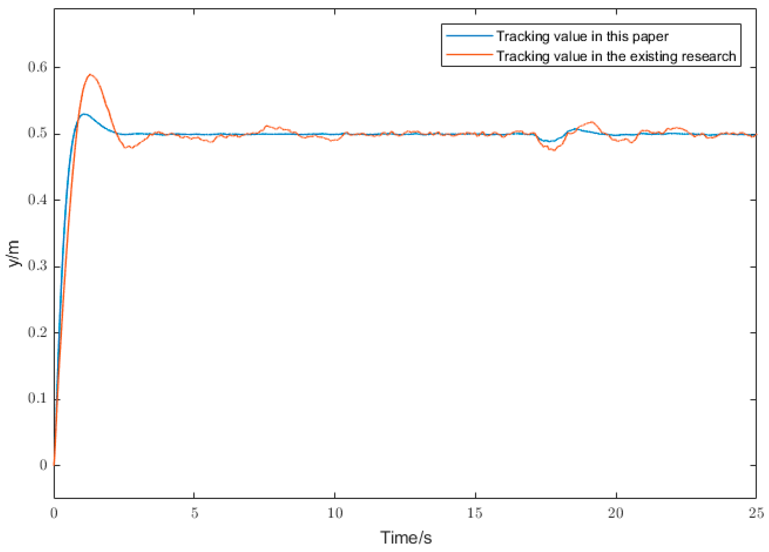
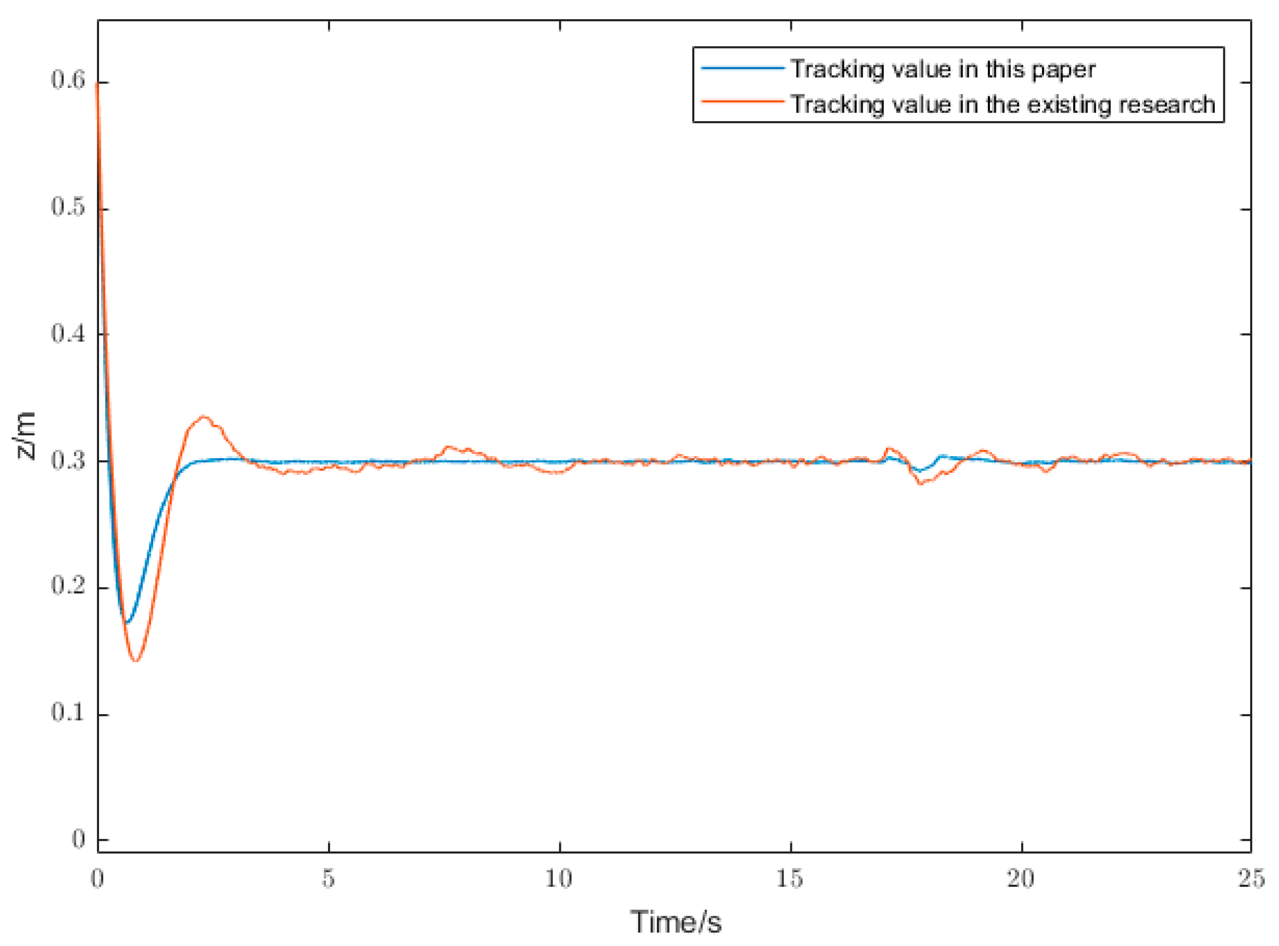
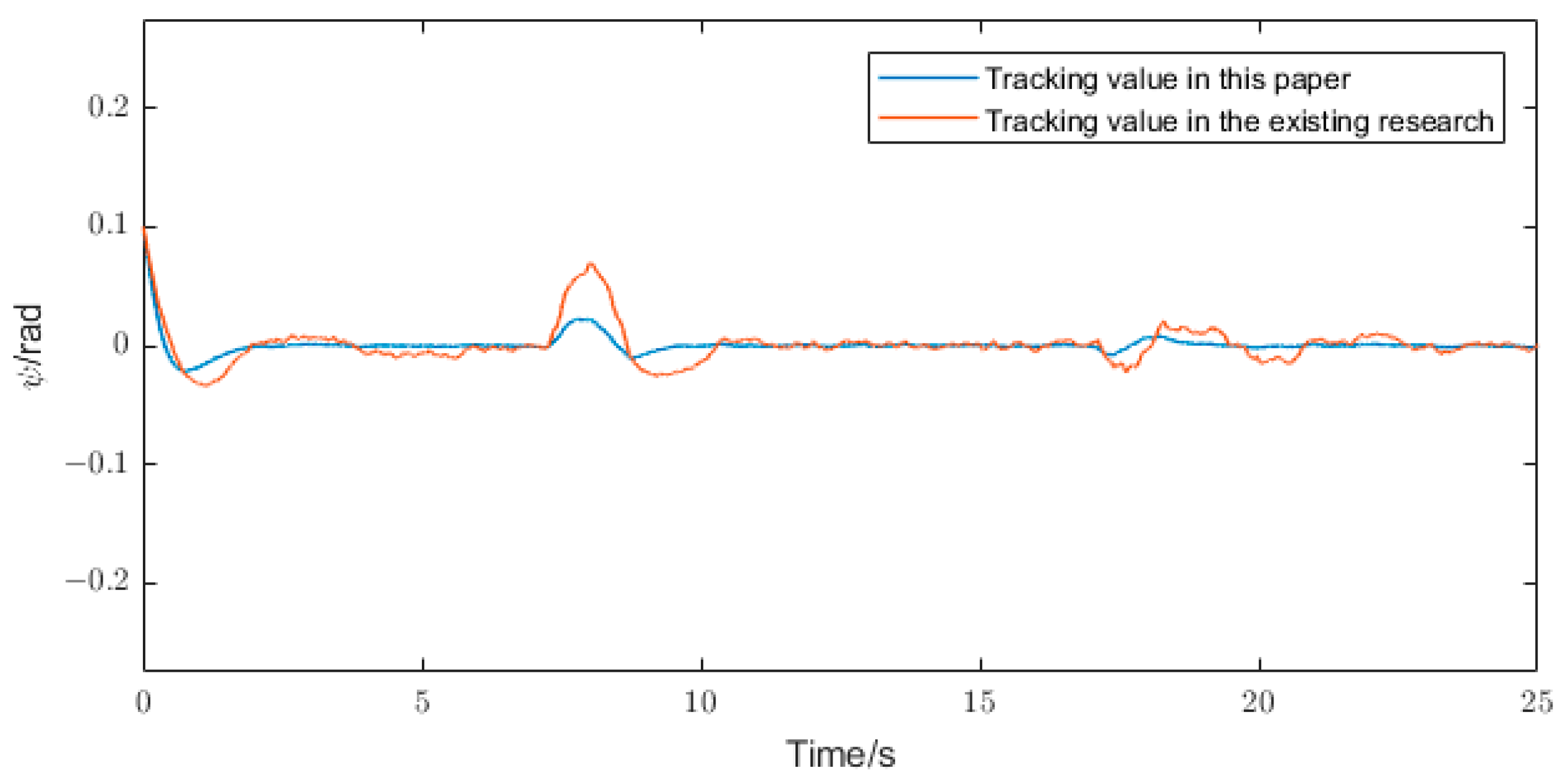
The initial condition of the aerial robot is set as , and the target condition is set as . The goal of control is to make the system reach the target position as soon as possible and steadily. At the 7th second of the experiment, 15% of the actuator failure is injected into the attitude control channel, and the robotic arm rotates between 17 and 21 s.
To determine whether the ANFTSMC approach in this paper has outstanding effects, this paper conducts a comparative experiment with the method proposed in [41].
It can be observed from Figure 7, Figure 8, Figure 9, Figure 10, Figure 11 and Figure 12 that the tracking value in this paper can reach the target position in about 2 s when there exist faults, and curves in this paper restore stability in about one second, which proves that the tracking errors are able to converge in finite time. When a fault occurs and the robotic arm is running, the proposed method and the sliding mode fault-tolerant control method in reference [41] can compensate for the fault information to make the system stable, but the comparison diagrams show that the trajectories in this article converge approximately 1 s faster than the trajectories in [41], and the convergence time of the proposed approach is shorter, reflecting the effectiveness of the fast convergence law. Meanwhile, the control method in this article can effectively weaken the chattering of the system compared with the other method.
Accordingly, the proposed FTC strategy has superior stability and a faster response speed.
6. Conclusions
This paper proposed an adaptive non-singular fast terminal sliding mode fault-tolerant control method based on an adaptive observer for aerial robot systems. When actuator faults occur in the system, the adaptive fault observer with anti-interference capability can estimate the time-varying faults accurately and weaken the chattering phenomenon. After defining the tracking error, a non-singular fast-reaching terminal sliding surface is designed. Considering various uncertain disturbances, including those caused by the rotation of the manipulator, several adaptive control laws are utilized to estimate the upper bounds of uncertain disturbances. By comparison with some existing FTC methods, it is obvious that the proposed approach has superior fault-tolerant performance. In future studies, we will focus on the uncertainty part of modeling in aerial robot systems.
Author Contributions
Conceptualization, P.Y.; methodology, P.Y. and Y.X.; validation, Y.X.; formal analysis, Y.X.; investigation, Y.X. and W.L.; writing—original draft preparation, Y.X.; writing—review and editing, Y.X. and W.L.; supervision, P.Y. All authors have read and agreed to the published version of the manuscript.
Funding
This work is supported by the National Natural Science Foundation of China (62273176), the Aeronautical Science Foundation of China (20200007018001), and the National Key Research and Development Program of China (2021YFB3301300).
Data Availability Statement
Data are contained within the article.
Conflicts of Interest
The authors declare no conflicts of interest.
References
- Freeman, M.R.; Kashani, M.M.; Vardanega, P.J. Aerial robotic technologies for civil engineering: Established and emerging practice. J. Unmanned Veh. Syst. 2021, 9, 75–91. [Google Scholar] [CrossRef]
- Zhou, Q.; Ding, S.; Qing, G.; Hu, J. UAV vision detection method for crane surface cracks based on Faster R-CNN and image segmentation. J. Civ. Struct. Health Monit. 2022, 12, 845–855. [Google Scholar] [CrossRef]
- Wu, D.; Zhang, W.; Du, H.; Wang, X. Robust adaptive finite-time trajectory tracking control of a quadrotor aircraft. Int. J. Robust Nonlinear Control 2021, 31, 8030–8054. [Google Scholar] [CrossRef]
- Lee, H.W. Research on multi-functional logistics intelligent Unmanned Aerial Vehicle. Eng. Appl. Artif. Intell. 2022, 116, 105341. [Google Scholar] [CrossRef]
- Dharmadhikari, M.; Dang, T.; Solanka, L.; Loje, J.; Nguyen, H.; Khedekar, N.; Alexis, S. Motion primitives-based path planning for fast and agile exploration using aerial robots. In Proceedings of the 2020 IEEE International Conference on Robotics and Automation (ICRA), Paris, France, 31 May–31 August 2020; IEEE: Piscataway, NJ, USA, 2020; pp. 179–185. [Google Scholar]
- Paul, H.; Miyazaki, R.; Ladig, R.; Shimonomura, K. TAMS: Development of a multipurpose three-arm aerial manipulator system. Adv. Robot. 2021, 35, 31–47. [Google Scholar] [CrossRef]
- Ollero, A.; Tognon, M.; Suarez, A.; Lee, D.; Franchi, A. Past, present, and future of aerial robotic manipulators. IEEE Trans. Robot. 2021, 38, 626–645. [Google Scholar] [CrossRef]
- Sinnemann, J.; Boshoff, M.; Dyrska, R.; Leonow, S.; Mönnigmann, M.; Kuhlenkötter, B. Systematic literature review of applications and usage potentials for the combination of unmanned aerial vehicles and mobile robot manipulators in production systems. Prod. Eng. 2022, 16, 579–596. [Google Scholar] [CrossRef]
- Khamseh, H.B.; Janabi-Sharifi, F.; Abdessameud, A. Aerial manipulation—A literature survey. Robot. Auton. Syst. 2018, 107, 221–235. [Google Scholar] [CrossRef]
- Pitla, S.; Bajwa, S.; Bhusal, S.; Brumm, T.; Brown-Brandl, T.M. Ground and Aerial Robots for Agricultural Production: Opportunities and Challenges; University of Nebraska: Lincoln, NE, USA, 2020. [Google Scholar]
- Zhao, M.; Okada, K.; Inaba, M. Versatile articulated aerial robot DRAGON: Aerial manipulation and grasping by vectorable thrust control. Int. J. Robot. Res. 2023, 42, 214–248. [Google Scholar] [CrossRef]
- Zhang, G.; He, Y.; Dai, B.; Gu, F.; Han, J.; Liu, G. Robust control of an aerial manipulator based on a variable inertia parameters model. IEEE Trans. Ind. Electron. 2020, 67, 9515–9525. [Google Scholar] [CrossRef]
- Jiao, R.; Chou, W.; Ding, R.; Dong, M. Adaptive robust control of quadrotor with a 2-degree-of-freedom robotic arm. Adv. Mech. Eng. 2018, 10, 1687814018778639. [Google Scholar] [CrossRef]
- Chaikalis, D.; Khorrami, F.; Tzes, A. Adaptive control approaches for an unmanned aerial manipulation system. In Proceedings of the 2020 International Conference on Unmanned Aircraft Systems (ICUAS), Athens, Greece, 1–4 September 2020; IEEE: Piscataway, NJ, USA, 2020; pp. 498–503. [Google Scholar]
- Zhiyuan, C.; Yanyang, L.; Yanhua, S.; Hongyu, C.; Bin, W.; Mingqi, H.; Rao, Y. Fuzzy sliding mode control for rotorcraft aerial manipulator with extended state observer. In Proceedings of the 2020 Chinese Automation Congress (CAC), Shanghai, China, 6–8 November 2020; IEEE: Piscataway, NJ, USA, 2020; pp. 1710–1714. [Google Scholar]
- Eneh, J.N.; Nwafor, S.C.; Nnadozie, E.C.; Ani, O.A. Adaptive Fuzzy Sliding Mode Control for an Aerial Manipulator as a Payload on a Quadcopter. In Proceedings of the 2022 5th Information Technology for Education and Development (ITED), Abuja, Nigeria, 1–3 November 2022; IEEE: Piscataway, NJ, USA, 2022; pp. 1–6. [Google Scholar]
- Chen, Y.; Liang, J.; Wu, Y.; Miao, Z. Adaptive sliding-mode disturbance observer-based finite-time control for unmanned aerial manipulator with prescribed performance. IEEE Trans. Cybern. 2022, 53, 3263–3276. [Google Scholar] [CrossRef] [PubMed]
- Hocaoglu, Y.; Mumcuoglu, M.E.; Unel, M. Disturbance observer based fault tolerant control of a quadrotor helicopter. In Proceedings of the IECON 2021–47th Annual Conference of the IEEE Industrial Electronics Society, Toronto, ON, Canada, 13–16 October 2021; IEEE: Piscataway, NJ, USA, 2021; pp. 1–6. [Google Scholar]
- Okada, K.F.Á.; de Morais, A.S.; Oliveira-Lopes, L.C.; Ribeiro, L. Neuroadaptive Observer-Based Fault-Diagnosis and Fault-Tolerant Control for Quadrotor UAV. In Proceedings of the 2021 14th IEEE International Conference on Industry Applications (INDUSCON), São Paulo, Brazil, 15–18 August 2021; IEEE: Piscataway, NJ, USA, 2021; pp. 285–292. [Google Scholar]
- Liu, K.; Yang, P.; Wang, R.; Jiao, L.; Li, T.; Zhang, J. Observer-based adaptive fuzzy finite-time attitude control for quadrotor UAVs. IEEE Trans. Aerosp. Electron. Syst. 2023, 59, 8637–8654. [Google Scholar] [CrossRef]
- Jiang, B.; Karimi, H.R.; Yang, S.; Gao, C.; Kao, Y. Observer-based adaptive sliding mode control for nonlinear stochastic Markov jump systems via T–S fuzzy modeling: Applications to robot arm model. IEEE Trans. Ind. Electron. 2020, 68, 466–477. [Google Scholar] [CrossRef]
- Seyedtabaii, S. New flat phase margin fractional order PID design: Perturbed UAV roll control study. Robot. Auton. Syst. 2017, 96, 58–64. [Google Scholar] [CrossRef]
- Wang, Y.; Shi, Y.; Cai, M.; Xu, W.; Yu, Q. Optimization of air–fuel ratio control of fuel-powered UAV engine using adaptive fuzzy-PID. J. Frankl. Inst. 2018, 355, 8554–8575. [Google Scholar] [CrossRef]
- Wang, B.; Zhang, W.; Zhang, L.; Zhang, Y. Adaptive fault-tolerant control of a quadrotor helicopter based on sliding mode control and radial basis function neural network. In Proceedings of the 2020 International Conference on Unmanned Aircraft Systems (ICUAS), Athens, Greece, 1–4 September 2020; IEEE: Piscataway, NJ, USA, 2020; pp. 832–838. [Google Scholar]
- Li, B.; Gong, W.; Yang, Y.; Xiao, B.; Ran, D. Appointed fixed time observer-based sliding mode control for a quadrotor UAV under external disturbances. IEEE Trans. Aerosp. Electron. Syst. 2021, 58, 290–303. [Google Scholar] [CrossRef]
- Shi, X.; Cheng, Y. Fuzzy adaptive sliding mode control for unmanned quadrotor. In Proceedings of the 2020 IEEE/ASME International Conference on Advanced Intelligent Mechatronics (AIM), Boston, MA, USA, 6–10 July 2020; IEEE: Piscataway, NJ, USA, 2020; pp. 1654–1658. [Google Scholar]
- Ullah, M.; Zhao, C.; Maqsood, H.; Nasir, A.; Humayun, M.; Hassan, M.U.; Alam, F. Adaptive Neural-Sliding Mode Control of a Quadrotor Vehicle with Uncertainties and Disturbances Compensation. In Proceedings of the 2022 2nd International Conference on Artificial Intelligence (ICAI), Islamabad, Pakistan, 30–31 March 2022; IEEE: Piscataway, NJ, USA, 2022; pp. 38–45. [Google Scholar]
- Hamadi, H.; Lussier, B.; Fantoni, I.; Francis, C.; Shraim, H. Comparative study of self-tuning, adaptive and multiplexing FTC strategies for successive failures in an Octorotor UAV. Robot. Auton. Syst. 2020, 133, 103602. [Google Scholar] [CrossRef]
- Nguyen, N.P.; Oh, H.; Moon, J. Continuous Nonsingular Terminal Sliding-Mode Control with Integral-Type Sliding Surface for Disturbed Systems: Application to Attitude Control for Quadrotor UAVs Under External Disturbances. IEEE Trans. Aerosp. Electron. Syst. 2022, 58, 5635–5660. [Google Scholar] [CrossRef]
- Lian, S.; Meng, W.; Shao, K.; Zheng, J.; Zhu, S.; Li, H. Full Attitude Control of a Quadrotor Using Fast Nonsingular Terminal Sliding Mode with Angular Velocity Planning. IEEE Trans. Ind. Electron. 2022, 70, 3975–3984. [Google Scholar] [CrossRef]
- Guo, Y.; Jiang, B.; Zhang, Y. A novel robust attitude control for quadrotor aircraft subject to actuator faults and wind gusts. IEEE CAAJ Autom. Sin 2017, 5, 292–300. [Google Scholar] [CrossRef]
- Eliker, K.; Zhang, W. Finite-time adaptive integral backstepping fast terminal sliding mode control application on quadrotor UAV. Int. J. Control. Autom. Syst. 2020, 18, 415–430. [Google Scholar] [CrossRef]
- Zhou, W.; Wang, X.; Wang, X.; Wang, W.; Liu, B. Design of sliding mode controller for tilting quadrotor UAV based on predetermined performance. J. Phys. Conf. Ser. 2021, 1748, 062074. [Google Scholar] [CrossRef]
- Jasim, O.A.; Veres, S.M. A robust controller for multi rotor UAVs. Aerosp. Sci. Technol. 2020, 105, 106010. [Google Scholar] [CrossRef]
- Ding, X.; Guo, P.; Xu, K.; Yu, Y. A review of aerial manipulation of small-scale rotorcraft unmanned robotic system. Chin. J. Aeronaut. 2019, 32, 200–214. [Google Scholar] [CrossRef]
- Cen, Z.; Noura, H.; Younes, Y.A. Systematic Fault Tolerant Control Based on Adaptive Thau Observer Estimation for Quadrotor Uavs. Int. J. Appl. Math. Comput. Sci. 2015, 25, 159–174. [Google Scholar] [CrossRef]
- Guo, J.; Qi, J.; Wu, C. Robust fault diagnosis and fault-tolerant control for nonlinear quadrotor unmanned aerial vehicle system with unknown actuator faults. Int. J. Adv. Robot. Syst. 2021, 18, 17298814211002734. [Google Scholar] [CrossRef]
- Zhang, K.; Jiang, B.; Cocquempot, V. Adaptive observer-based fast fault estimation. Int. J. Control Autom. Syst. 2008, 6, 320–326. [Google Scholar]
- Jin, X. Adaptive fixed-time control for MIMO nonlinear systems with asymmetric output constraints using universal barrier functions. IEEE Trans. Autom. Control 2018, 64, 3046–3053. [Google Scholar] [CrossRef]
- Wu, Y.; Zhang, G.; Wu, L. Observer-based adaptive fault estimation and fault-tolerant tracking control for a class of uncertain nonlinear systems. IET Control Theory Appl. 2021, 15, 13–23. [Google Scholar] [CrossRef]
- Ding, Y.; Wang, X.; Bai, Y.; Cui, N. Global smooth sliding mode controller for flexible air-breathing hypersonic vehicle with actuator faults. Aerosp. Sci. Technol. 2019, 92, 563–578. [Google Scholar] [CrossRef]
Figure 1.
Model of the aerial robot.

Figure 2.
Aerial robot.

Figure 3.
Spatial positioning system.

Figure 4.
Ground workstation.

Figure 5.
Estimated value comparison diagram in situation 1.

Figure 6.
Estimated value comparison diagram in situation 2.

Figure 7.
Tracking values of .

Figure 8.
Tracking values of .

Figure 9.
Tracking values of .

Figure 10.
Tracking values of .

Figure 11.
Tracking values of .

Figure 12.
Tracking values of .


Table 1.
Parameters of the aerial robot.
| Symbol | Implication | Numerical Value |
|---|---|---|
| Quality of the aerial robot | ||
| Arm length of UAV | 0.54 m | |
| Rotational inertia around axis | ||
| Rotational inertia around axis | ||
| Rotational inertia around axis | ||
| Acceleration of gravity |
Table 2.
Controller parameters.
| Parameters | Value |
|---|---|
| 10 | |
| 50 | |
| 1.4 | |
| 0.6 | |
| 0.5 | |
| 0.5 | |
| 0.5 | |
| 2 |
Disclaimer/Publisher’s Note: The statements, opinions and data contained in all publications are solely those of the individual author(s) and contributor(s) and not of MDPI and/or the editor(s). MDPI and/or the editor(s) disclaim responsibility for any injury to people or property resulting from any ideas, methods, instructions or products referred to in the content. |
© 2024 by the authors. Licensee MDPI, Basel, Switzerland. This article is an open access article distributed under the terms and conditions of the Creative Commons Attribution (CC BY) license (https://creativecommons.org/licenses/by/4.0/).
Share and Cite
MDPI and ACS Style
Yang, P.; Xuan, Y.; Li, W. Adaptive Nonsingular Fast-Reaching Terminal Sliding Mode Control Based on Observer for Aerial Robots. Actuators 2024, 13, 98. https://doi.org/10.3390/act13030098
AMA Style
Yang P, Xuan Y, Li W. Adaptive Nonsingular Fast-Reaching Terminal Sliding Mode Control Based on Observer for Aerial Robots. Actuators. 2024; 13(3):98. https://doi.org/10.3390/act13030098
Chicago/Turabian StyleYang, Pu, Yan Xuan, and Wanting Li. 2024. "Adaptive Nonsingular Fast-Reaching Terminal Sliding Mode Control Based on Observer for Aerial Robots" Actuators 13, no. 3: 98. https://doi.org/10.3390/act13030098
Note that from the first issue of 2016, this journal uses article numbers instead of page numbers. See further details here.