Article

Dynamic Modeling, Simulation, and Optimization of Vehicle Electronic Stability Program Algorithm Based on Back Propagation Neural Network and PID Algorithm

College of Mechanical and Energy Engineering, Beijing University of Technology, Beijing 100124, China
*
Author to whom correspondence should be addressed.
These authors contributed equally to this work.
Actuators 2024, 13(3), 100; https://doi.org/10.3390/act13030100
Submission received: 2 January 2024 / Revised: 15 February 2024 / Accepted: 26 February 2024 / Published: 4 March 2024
(This article belongs to the Section Actuators for Land Transport)

Abstract

:
The vehicle lateral stability control algorithm is an essential component of the electronic stability program (ESP), and its control effect directly affects the vehicle’s driving safety. However, there are still numerous shortcomings and challenges that need to be addressed, including enhancing the efficiency of processing intricate pavement condition data, improving the accuracy of parameter adjustment, and identifying subtle and elusive patterns amidst noisy and ambiguous data. The introduction of machine learning algorithms can address the aforementioned issues, making it imperative to apply machine learning to the research of lateral stability control algorithms. This paper presented a vehicle lateral electronic stability control algorithm based on the back propagation (BP) neural network and PID control algorithm. Firstly, the dynamics of the whole vehicle have been analytically modeled. Then, a 2 DOF prediction model and a 14 DOF simulation model were built in MATLAB Simulink to simulate the data of the electronic control units (ECU) in ESP and estimate the dynamic performance of the real vehicle. In addition, the self-correction of the PID algorithm was verified by a Simulink/CarSim combined simulation. The improvement of the BP neural network to the traditional PID algorithm was also analyzed in Simulink. These simulation results show the self-correction of the PID algorithm on the lateral stability control of the vehicle under different road conditions and at different vehicle speeds. The BP neural network smoothed the vehicle trajectory controlled by traditional PID and improved the self-correction ability of the control system by iterative training. Furthermore, it shows that the algorithm can automatically tune the control parameters and optimize the control process of the lateral electronic stability control algorithm, thus improving vehicle stability and adapting it to many different vehicle models and road conditions. Therefore, the algorithm has a high practical value and provides a feasible idea for developing a more intelligent and general vehicle lateral electronic stability system.

1. Introduction

Since the invention and validation of ESP at the beginning of this century [1], it has been widely used in the automotive industry and has now become one of the most important research fields. In recent years, with the rise of autonomous vehicles, there has been a lot of in-depth research on their motion control [2,3], safety performance [4,5], and stability [6]. However, it is challenging to achieve a balance between mobility, safety, and stability [7]. Therefore, a highly robust ESP that can simultaneously address the other two requirements is essential. In addition, the control algorithm of ESP for lateral stability needs more in-depth improvement and perfection.
Before any control algorithm is put into practical applications, it must be modeled theoretically to gain a deep understanding and validated by numerical simulations to reduce the high cost of practical testing [8]. The low-DOF model is used to capture the characteristics of the idealized control target of the vehicle, including other secondary parameters, such as slip angle [9,10,11,12,13], yaw angle [9,13,14], and yaw torque [15,16]. Gang et al. [10] developed a 4 DOF model to describe the steering stability of the vehicle by calculating the slip angle, thus verifying the effectiveness of the differential algorithm. Peng et al. [14] used 2 DOF models to calculate the yaw angle and analyzed the steady- and transient-state of the vehicle lateral stability to validate the slip steering technique. Liang et al. [15] also established a 2 DOF model to understand the driving dynamics and steering stability of the vehicle by calculating the yaw moment and verified the advantages of the genetic algorithm over the traditional PID algorithm. The high DOF models are used to realistically simulate a wide range of vehicle performance in real-world driving, such as handling performance [17,18,19] and dynamic performance [13,20,21,22]. Ni et al. [17] developed an 11 DOF vehicle dynamics model to simulate the handling performance of a hybrid eight-wheel drive vehicle by modeling and correlating each part of the complex vehicle system. Yu et al. [20] developed a 14 DOF vehicle model based on Lagrange’s equations to describe the enhanced dynamic and energy efficiency performance of an electric vehicle with four independent wheel drives.
The control algorithm is the key to ensuring the lateral stability of the vehicle in driving, the algorithm for vehicle stability has emerged in recent years, mainly from two aspects to optimize the control effect of vehicle stability: self-adaptability and fast response. The optimization can be achieved by introducing a new additional controller to assist the control algorithm [23,24,25,26,27,28,29,30] or by optimizing the control algorithm itself [31,32,33,34,35,36,37,38], which enables the vehicle to respond to more road conditions and enhances its stability. Yuan et al. [25] introduced a new electronically stable controller based on the Mu control theory [39], which improved the robustness and stability of the vehicle by reducing external disturbances. Yu et al. [32] developed a new control architecture based on slip ratio control and direct yaw moment control by estimating the traction force when the tires are driven in a straight line. The optimization of control systems [25,32] enables the vehicle to respond to more road conditions and enhances its stability. To improve the responsiveness, Jin et al. [29] introduced the logic gate control to the PID control algorithm to maneuver the vehicle by tuning the PID parameters through the logic gate algorithm, thus improving the algorithm efficiency. Cho et al. [36] reduced the computational cost of the vehicle ECU by using an integrated logical framework to optimize the overall structure of the algorithm, increasing the response speed and thus stabilizing the vehicle. Most of the existing studies mainly rely on traditional control algorithms to realize vehicle stability control. However, traditional control algorithms are poorly adapted to nonlinear and time-varying systems, sensitive to parameter changes, and not applicable to multivariable systems. The introduction of machine learning can improve the robustness of the algorithms for nonlinear systems, as well as parameter optimization. There are also many challenges in combining neural networks and traditional control algorithms, such as how to utilize neural networks to regulate the parameters of traditional control algorithms, and how the configuration of neural networks can be adapted to combine with traditional control algorithms. The integration of traditional control methods with emerging machine learning techniques applied to vehicle stability control has the potential to elevate the efficiency and effectiveness of vehicle stability control systems to new levels.
In this paper, a prediction model and a simulation model of the vehicle are established through dynamics analysis. A new lateral stability control algorithm is proposed by combining the PID and BP neural network algorithm. Its control effect is estimated by simulations. To simulate the ideal data in the MCU and the real driving condition of the vehicle, we establish a MATLAB Simulink model based on a 2 DOF analytical prediction and a 14 DOF numerical model. Then, through the combination of the PID algorithm and BP neural network algorithm, a vehicle lateral electronic stability control algorithm that can automatically adjust the control parameters and optimize the control process was proposed and simulated. Meanwhile, the simulation data was used to verify that the PID algorithm can improve vehicle stability by correcting the yaw rate under different road conditions. Also, the simulation data can verify that the PID algorithm can be optimized by iterative training of the BP neural network. The combination of the BP neural network and PID algorithm can dynamically adjust the parameters of the PID algorithm to improve the control effect. The results show that the algorithm can effectively improve the stability of the vehicle in more road conditions and can make the control effect smoother, effectively avoiding the occurrence of accidents.

2. Methods

The ECU of the ESP mainly consisted of a processing microcontroller unit (MCU), a motion control MCU, a data communication module, a module driving a solenoid valve, and a module driving a hydraulic pump motor, which is responsible for computing and processing. The main function of the processing MCU is to read and analyze the sensor data and calculate the current vehicle driving data. When the actual data during driving deviates from the target data determined by the ESP system, the processing MCU will call the pre-set stability control algorithm, calculate the corresponding correction command by the current vehicle conditions, and send it to the motion control MCU (Figure 1).
In this study, the analytical predictive and numerical simulation models were established to analyze the yaw motion of a vehicle. First, the predictive model running in the MCU calculated the theoretical state of vehicles and compared it with the data from the yaw rate sensor and wheel speed sensor to determine whether the vehicle was unstable. Then, the simulation model simulated the real vehicle and the external environment, which was combined with the predictive model to test and verify the ESP stabilization algorithm and in turn, make corrections to the ESP based on the simulation results.

2.1. Predictive Model

The 2-degree of freedom (DOF) dynamics model is simple to calculate, suitable for operation in an MCU, and can adequately reflect the yaw motion of the vehicles. Since it ignores most other effects and only considers the yaw motion, it reflects the yaw rate change when the vehicle is steering in the ideal state while meeting the requirements of prediction accuracy. Therefore, it is very suitable for generating target values as a prediction model.
Figure 2 shows a 2-DOF dynamics model based on the structure of the simulated vehicle. The model only took the angle of rotation of the front wheels as input and ignored the influence of the steering system and the suspension, assuming that the vehicle’s forward speed u is constant. It is assumed that the vehicle simply moved in a 2D plane relative to the ground. The model was used to solve for the idealized yaw rate of the vehicle and the change in the lateral deflection angle of the center of mass.
The kinematic analysis of the 2-DOF dynamics model was established. The model is simplified as a lumped mass. Parameters such as the vehicle’s rotational inertia and mass distribution coefficient can be considered as being constants, which makes it easier to establish the governing equations of motion, which were obtained by decomposing the external forces and moments of the vehicle as well as the absolute velocity and angular acceleration of the vehicle along the axes of the coordinate system (Figure 3).
ax and ay are the x- and y- components of the acceleration of the center of mass of the vehicle, respectively. At time t, the x- and y- components of the velocity v′ of the center of mass are u and v, while at t + Δt, the velocity of the center of mass is changed because of the coordinate transformation in Equation (1).
u + Δ u cos Δ θ u v + Δ v sin Δ θ = u cos Δ θ + Δ u cos Δ θ u v sin Δ θ Δ v sin Δ θ
where Δθ is the angle of transformation between the old and new coordinate system; Δθ is a small angle, using small-angle approximation and neglecting second-order trace, the above equations can be rewritten as Equation (2).
u + Δ u cos Δ θ u v + Δ v sin Δ θ = Δ u v Δ θ
Dividing by Δt and taking the limit, the formula for the component of the absolute acceleration of the vehicle in the x-direction was obtained.
a x = lim Δ t 0 Δ u Δ t v lim Δ t 0 Δ θ Δ t = d u d t v d θ d t = u ˙ v ω r
where ωr is the yaw rate of the vehicle, where ωr = dθ/dt. Similarly, the absolute acceleration of the vehicle was calculated as y-component.
a y = v ˙ + u ω r
Figure 1 shows the 2-DOF model. The vehicle was subjected to the net forces along the y-axis and the net moments around the center of mass. Fy1 and Fy2 are the lateral reactions exerted by the ground on the front wheel and rear wheel, respectively. A and B are the distance from the front wheel to the center of mass and the rear wheel to the center of mass, respectively. η is a small angle, using the small-angle approximation of the net force, and the combined moments are given in Equations (5) and (6).
F y = F y 1 cos η + F y 2 = F y 1 + F y 2 = k 1 α 1 + k 2 α 2
M z = A F y 1 cos η B F y 2 = A F y 1 B F y 2 = A k 1 α 1 B k 2 α 2
where k1 and k2 are the lateral deflection stiffness of the front wheel and rear wheel, respectively. α1 and α2 are the lateral deflection angles of the front wheel and rear wheel, respectively. Equations are given in Equations (7) and (8) based on the geometric relationship (Figure 1)
β tan β = v u
λ tan λ = v + A ω r u
where β is the lateral declination of the center of mass; λ is the angle between the direction of the velocity of the front wheel and the x-direction; both β and λ are small angles; v is the y-component of the velocity of the center of mass; and u is the x-component of the velocity of the center of mass (the vehicle’s forward speed). Based on the geometric relationship in Figure 1 and Equations (7) and (8), and considering α1 and α2 clockwise as positive and counterclockwise as negative, the lateral eccentricity angle of the front and back masses is given in Equation (9).
α 1 = η λ = β + A ω r u η
α 2 = v B ω r u = β B ω r u
where B is the distance from the rear wheel to the center of mass. Substituting Equations (9) and (10) into (5) and (6) yields
F y = k 1 β + A ω r u η + k 2 β B ω r u
M z = A k 1 β + A ω r u η + B k 2 β B ω r u
Considering inertia force, the differential equation of motion for the 2-DOF vehicle model is given as
m v ˙ + u ω r = k 1 β + A ω r u δ + k 2 β B ω r u
I z ω ˙ r = A k 1 β + A ω r u δ + B k 2 β B ω r u
where Iz is the moment of inertia of the vehicle around the z-axis. Equations (13) and (14) can be rewritten as Equations (15) and (16).
ω ˙ r = A 2 k 1 B 2 k 2 I z u ω r + A k 1 B k 2 I z β A k 1 I z η
β ˙ = A k 1 B k 2 m u 2 1 ω r + k 1 + k 2 m u β k 1 m u η
which can be expressed in the standard form of a state-space equation.
ω ˙ r γ ˙ = a 11 a 12 a 21 a 22 ω r γ + b 11 b 21 η
ω r γ = 1 0 0 1 ω r γ + 0 0 η
where a 11 = p 2 k 1 + q 2 k 2 I z u , a 12 = p k 1 q k 2 I z , a 21 = p k 1 + q k 2 m u 2 1 , a 22 = k 1 + k 2 m u , b 11 = p k 1 I z , b 21 = k 1 m u .
Figure 4 shows the predictive model built in MATLAB Simulink using the standard state-space equation approach.

2.2. Simulation Model

If vehicle behavior is not predicted at the time of designing a vehicle, it may lead to improper handling behavior and hazards. However, since the cost of conducting real vehicle experiments is too high, it is necessary to simulate the dynamic behavior and safety of real vehicles through computer and mathematical models [40]. The 14-DOF model provides a better representation of the lateral and yaw dynamics of the vehicle compared to the low degree of freedom model. It takes into account the suspension at each corner and has the capability of predicting the pitching and heave motion of the vehicle [41]. The 14-DOF automobile dynamics model is divided into a 7-DOF suspension model and a 7-DOF handling model. It contains 6-DOF for the translation and rotation of the car body along the x-axis, y-axis, and z-axis, and 4-DOF for the vertical movement of the four suspensions and 4 DOFs for the rotation of the wheels.
First, the pitch and lateral motion of the vehicle were analyzed. When the vehicle is steered, the body is rotated around the z-axis, but also undergoes a pitching motion along the y-axis, and Figure 5 shows a lateral motion along the x-axis because of inertia.
The kinetic equation for the pitching motion of the vehicle on the y-axis is
I s y θ ¨ = m s a x h + m s g h θ k θ θ β θ θ ˙
where Isy is the moment of inertia of the vehicle’s spring-loaded mass around the y-axis; h is the height of the vehicle’s spring-loaded mass from the ground; kθ is the vehicle’s pitch motion stiffness factor; βθ is the vehicle’s pitch motion damping factor; θ is the pitch angle.
The kinetic equation for the lateral motion of the vehicle along the x-axis is
I r + m s h h r c cos ϕ 2 ϕ ¨ = m s a y h h r c + m s g h h r c tan ϕ k ϕ ϕ β ϕ ϕ ˙
where Ir is the moment of inertia of the vehicle’s spring-loaded mass around the x-axis; h is the height of the vehicle’s center of mass from the ground; hrc is the height of the vehicle’s center of sway from the ground; kϕ is the vehicle’s lateral motion stiffness factor; βϕ is the vehicle’s lateral motion damping factor; and ϕ is the lateral angle.
Then, the forces in the lead director of the vehicle were analyzed, the suspension of the vehicle was simplified to a first-order spring damping system, and the tires of the vehicle were simplified to a spring-slider model fixed to the ground. The suspension and tires were moved along the lead director, with a total of 4-DOF, and the spring-loaded mass can do translational movement along the lead direction and rotation around the x- and y- axes, with a total of 3-DOF. Figure 6 shows the simplified 7-DOF suspension model.
The equation was based on Newton’s second law and Newton’s second law for rotation. Along the z-axis, the equation of motion in the lead direction is
F s f l + F d f l + F s f r + F d f r + F s r l + F d r l + F s r r + F d r r = m s Z ¨ s
In the direction of rotation around the y-axis, the equation of pitch motion is
F s r l + F d r l + F s r r + F d r r b F s f l + F d f l + F s f r + F d f r a = I y θ ¨
In the direction of rotation around the x-axis, the equation of lateral motion is
F s f l + F d f l + F s r l + F d r l w 2 F s f r + F d f r + F s r r + F d r r w 2 = I x ϕ ¨
where Fsfl, Fsfr, Fsrl, and Fsrr are the vehicle suspension spring force of the left front, right front, left rear, and right rear; Fdfl, Fdfr, Fdrl, and Fdrr are the vehicle suspension damping force of the left front, right front, left rear and right rear; a is the vehicle front wheel to the center of mass distance; b is the vehicle rear wheel to the center of mass distance; w is the vehicle width; ms is the vehicle spring load mass; Iy and Ix are the moment of inertia of the vehicle’s spring-loaded mass around the y-axis and the x-axis; Zs is the displacement of the vehicle’s spring-loaded mass along the z-axis; θ is the angle of rotation of the vehicle’s spring-loaded mass along the y-axis (the pitch angle) in Figure 5; and ϕ is the angle of rotation of the vehicle’s spring-loaded mass along the x-axis (the lateral angle) in Figure 5.
The equation of motion in the lead director of the four wheels is as follows:
F t f l F s f l F d f l = m u f l Z ¨ u f l F t f r F s f r F d f r = m u f r Z ¨ u f r F t r l F s r l F d r l = m u r l Z ¨ u r l F t r r F s r r F d r r = m u r r Z ¨ u r r
where Ftfl, Ftfr, Ftrl, and Ftrr are the vehicle’s tire elasticity of the left front, right front, left rear, and right rear; mufl, mufr, murl, and murr are the vehicle’s suspension mass of the left front, right front, left rear and right rear; and Zufl, Zufr, Zurl, and Zurr are the vehicle’s suspension displacement along the z-axis of the left front, right front, left rear and right rear. The vehicle’s four-wheel load can be obtained by the following equation:
F z f l = m s g b 2 a + b + m u f l g + F s f l + F d f l F z f r = m s g b 2 a + b + m u f r g + F s f r + F d f r F z r l = m s g a 2 a + b + m u r l g + F s r l + F d r l F z r r = m s g a 2 a + b + m u r r g + F s r r + F d r r
where Fzfl, Fzfr, Fzrl, and Fzrr are the wheel load of the left front, right front, left rear, and right front. On the right side of Equation (25), the first part represents the body mass component, the second part represents the wheel mass, the third part represents the suspension spring force component, and the fourth part represents the suspension damping force component; ms is the body mass.
After completing the suspension model, control variables such as current vehicle speed and front-wheel angle input are associated with the model to create a manipulation model of the vehicle. The vehicle manipulation model contains 2-DOF for translational movement along the x- and y- axes, 1 DOF for rotation around the z-axis, and 4-DOF for the rotation of the wheels. Figure 7 shows the simplified 7-DOF manipulation model built in MATLAB Simulink.
Regarding the kinematic analysis of the 7-DOF manipulation model, as analyzed previously when building the 2-DOF model, from Equations (1)–(4), the calculation results are given in Equation (26).
a x = v ˙ x v y ψ ˙ a y = v ˙ y + v x ψ ˙
where ax and ay are the acceleration of the vehicle along the x-axis and the y-axis; vx and vy are the speed of the vehicle along the x-axis and the y-axis; and ψ is the angle of rotation of the vehicle along the z-axis.
The kinetic equation for the longitudinal motion of the vehicle along the x-axis is
F x f l cos δ F y f l sin δ + F x f r cos δ F y f r sin δ + F x r l + F x r r = m t a y
The kinetic equation for the lateral motion of the vehicle along the y-axis is
F y f l cos δ + F x f l sin δ + F y f r cos δ + F x f r sin δ + F y r l + F y r r = m t a y
where Fxfl, Fxfr, Fxrl, and Fxrr are the force along the x-axis on the wheel of left front, right front, left rear, and right rear; Fyfl, Fyfr, Fyrl, and Fyrr are the force along the y-axis on the wheel of left front, right front, left rear, and right rear; mt is the mass of the vehicle; and δ is the angle of rotation of the front wheel.
When the vehicle is steered, the kinetic equation for the vehicle’s rotation around the z-axis is
w 2 F x f l cos δ + w 2 F x f r cos δ w 2 F x r l + w 2 F x r r + w 2 F y f l sin δ w 2 F y f r sin δ + a F x f l sin δ + a F y f l cos δ + a F x f r sin δ + a F y f r cos δ b F y r l b F y r r + M z f l + M z f r + M z r l + M z r r = J z ψ ¨
where Mzfl, Mzfr, Mzrl, and Mzrr are the moment around the z-axis of the left front wheel, the right front wheel, the left rear wheel, and the right rear wheel; w is the center distance between the left and right tires of the vehicle.
Finally, the first step of building the tire model is to calculate the slip angle of the tire. Slip angle is the angle between the direction of travel of the vehicle and the direction of the tires and was calculated in Figure 7.
α f l = tan 1 v y + a ψ ˙ v x 0.5 w ψ ˙ δ α f r = tan 1 v y + a ψ ˙ v x + 0.5 w ψ ˙ δ α r l = tan 1 v y b ψ ˙ v x 0.5 w ψ ˙ α r r = tan 1 v y b ψ ˙ v x + 0.5 w ψ ˙
where αfl, αfr, αrl, and αrr are the slip angle of the left front wheel, the right front wheel, the left rear wheel, and the right rear wheel; δ is the angle of rotation of the front wheel (Figure 7).
The formula for calculating the speed of the four wheels of a vehicle is as follows:
V w x f l = cos α f l v y + a ψ ˙ 2 + v x 0.5 w ψ ˙ 2 V w x f r = cos α f r v y + a ψ ˙ 2 + v x + 0.5 w ψ ˙ 2 V w x r l = cos α r l v y b ψ ˙ 2 + v x 0.5 w ψ ˙ 2 V w x r r = cos α r r v y b ψ ˙ 2 + v x + 0.5 w ψ ˙ 2
where Vwxfl, Vwxfr, Vwxrl, and Vwxrr are the speeds of the left front wheel, the right front wheel, the left rear wheel, and the right rear wheel.
The forces on the tire were analyzed, and the tire was subjected to driving torque from the engine in the direction of rotation, braking torque from the brake caliper, and frictional force from the ground.
I w ω ˙ f l = T d f l T b f l F x f l R w I w ω ˙ f r = T d f r T b f r F x f r R w I w ω ˙ r l = T d r l T b r l F x r l R w I w ω ˙ r r = T d r r T b r r F x r r R w
where Iw is the moment of inertia of the wheels of the vehicle; Rw is the radius of the wheels of the vehicle; ωfl, ωfr, ωrl, and ωrr are the speed of the left front wheel, the right front wheel, the left rear wheel, and the right rear wheel; Tdfl, Tdfr, Tdrl, and Tdrr are the drive torque of the left front wheel, the right front wheel, the left rear wheel, and the right rear wheel; Tbfl, Tbfr, Tbrl, and Tbrr re the braking torque of the left front wheel, the right front wheel, the left rear wheel, and the right rear wheel; and Fxfl, Fxfr, Fxrl, and Fxrr are the friction applied to the left front wheel, the right front wheel, the left rear wheel, and the right rear wheel. Combining Equations (30)–(32), thespeed change rate of each wheel is given in Equation (33).
S a f l = V w x f l ω f l R w V w x f l S a f r = V w x f r ω f r R w V w x f r S a r l = V w x r l ω r l R w V w x r l S a r r = V w x r r ω r r R w V w x r r
where Safl, Safr, Sarl, and Sarr are the speed change rates of the left front wheel, the right front wheel, the left rear wheel, and the right rear wheel.
According to the magic formula proposed by H.B. Pacejke [42], the pitch force Fx calculation formula (Equation (33)) was obtained by fitting the tire test data in the combined formula of trigonometric functions i and the tire force.
F x = D x sin C x arctan B x X 1 E x B x X 1 arctan B x X 1
Lateral forces Fy calculation formula
F y = D y sin C y arctan B y X 2 E y B y X 2 arctan B y X 2
Return torque Mz calculation formula
M z = D z sin C z arctan B z X 3 E z B z X 3 arctan B z X 3
where X is the lateral deflection angle or pitch slip rate; D is the peak factor; B is the stiffness factor; C is the curve shape factor; and E is the curve curvature factor. The hyperparameters that appear in Equations (34)–(36) can be obtained from Table 1.
The 14-DOF vehicle dynamics model has a complex structure related to many internal variables, thus it is hard to establish clear standard state-space equations like the 2-DOF model, and each sub-system sub-module needs to be modeled separately and then associated with each other. Finally, the 7-DOF suspension model, the 7-DOF manipulation model, and the tire model are associated, and Figure 8 shows the 14-DOF vehicle dynamics model built on this basis in MATLAB Simulink.

2.3. Validation of the Simulation Model

At a vehicle speed of 80 km/h, after a response time from t = 0 s to t = 1.5 s, the simulator turns the steering wheel 180 degrees to the right from t = 1.5 s to t = 2 s and stays. Figure 9 shows a comparison of the measured yaw rate profiles of the predictive model and the simulation model at a speed of 80 km/h.
The comparison results show that there is still a large difference between the output of the simulation model and the prediction model, although for the same vehicle speed and the same steering wheel angle input. The simulation model uses a 14-DOF model with inputs that contain more influences and are closer to the real situation and are referred to as actual values. A 2-DOF model is used to generate the target value for the control variables, where the 2-DOF model ignores most of the perturbations that are closer to the ideal situation. The ESP determines the operating state of the vehicle by comparing the actual value with the target value and then invokes the lateral stability control algorithm to control the body stability according to the difference between the target and actual values.

3. PID Lateral Stability Control Algorithm

After studying various vehicle electronic stability control algorithms and simulation validation methods, it was determined that the accuracy of the mathematical model of the vehicle and the effectiveness of the vehicle’s lateral stability control system can be verified through joint simulation using the PID control algorithm.

3.1. PID Algorithm Controller Model

This simulation aims to verify the effectiveness of using the PID algorithm as a vehicle lateral electronic stability control algorithm. The process needs to reduce perturbations, and on balance, a joint simulation using MATLAB Simulink and CarSim is more suitable. This method is highly authentic, and the simulation results are more accurate and convenient to obtain.
A real-time vehicle model is developed in the CarSim2019 software platform and is linked to the control model in the MATLAB R2020a Simulink, as shown in Figure 10a. The established 2-DOF and PID control models were introduced into the electronic stability controller module (Figure 10b). The simulated lateral electronic stability control model was established, where Kp is the scaling factor; Ki is the integral adjustment factor; and Kd is the differential adjustment factor. The PID algorithm dynamically adjust the system by tuning the Kp and Ki, and Kd. e(t) to the actual value. u(t) is the output signal of the PID algorithm model.

3.2. PID Algorithm Validation Methods

There are many test methods for the ESP. This study combines the steering wheel input method of the sine-dwell test and the evaluation criteria of the double-lane change test and improves the test method for the lateral stability system of vehicles following the characteristics of the computer simulation environment. The improved test procedure is as follows: after a response time from t = 0 s to t = 1 s, the simulator turns the steering wheel 180 degrees to the right from t = 1 s to t = 1.5 s, then stays from t = 1.5 s to t = 2 s, then turns the steering wheel 360 degrees to the right from t = 2 s to t = 3 s, then stays from t = 3 s to t = 4.5 s, then turns the steering wheel 360 degrees to the right from t = 4.5 s to t = 5.7 s, and then stays from 5.7 s to 6.2 s, at last returning to 0 degrees from 6.2 s to 6.7 s. Tests were performed with a normal road friction coefficient of 1.0 and a low adhesion road friction coefficient of 0.5.
The test was performed with the initial speed measurement as the variable, starting at 40 km/h and increasing by 5 km/h each time, without throttle or brake action during the test. For each speed level, a simulation of the vehicle without and with lateral stability control intervention was tested and the yaw rate profile of the vehicle was recorded. The yaw rate curves were compared for each group and the effect of the vehicle lateral stability control on the body movement under normal road conditions and low adhesion road conditions were analyzed.

4. BP Neural Network-Based PID Lateral Stability Control Algorithm

ESP plays a pivotal role in enhancing vehicle stability and reducing crashes, and has always been a cornerstone of automotive safety. Despite advances in control technology, conventional algorithms often struggle to cope with the complexities inherent in dynamic driving environments. These challenges arise from the nonlinear nature of vehicle dynamics, as well as a variety of factors such as driver behavior, weather conditions, and road surfaces. In contrast, emerging technologies, especially machine learning, offer promising ways to address these shortcomings. Artificial neural network technology, in particular, has shown a remarkable ability to handle the intricate control and decision-making tasks posed by complex systems. By utilizing the inherent nonlinear mapping ability and flexible network structure of neural networks, we can develop more adaptive and self-tuning algorithms for lateral stability control of ESP systems. BP neural networks, known for their robust performance in nonlinear systems, are suitable candidates for enhanced lateral stability control algorithms. Combining BP neural networks with conventional PID control algorithms holds great potential for creating adaptive ESP systems that can automatically adapt to various driving conditions. These advances are expected to not only improve vehicle safety but also pave the way for wider adoption of ESP systems.

4.1. BP Neural Network-Based PID Algorithm Controller Model

A MATLAB Simulink simulation model based on the BP neural network was developed for the theory and characteristics of the vehicle lateral stability controller.
The BP neural network-based PID controller is similar in structure to the established PID controller. The established simulation model of the vehicle’s 2-DOF dynamics was chosen as the prediction model, and the target yaw rate profile generated by it was used as the control signal r(k). The controlled system model was used to simulate the actual operation of the vehicle. To meet the requirements of the iterative training speed of the BP neural network and the flexibility of defining various variables, the established 14-DOF vehicle dynamics validation model was used as the controlled system and the actual yaw rate profile generated by it was used as the feedback signal y(k). e(k) is r(k) − y(k) and u(k) is the regulation signal obtained after the operation of the PID control algorithm. The PID algorithm regulation process is expressed in the form of an incremental digital PID control equation as follows
u ( k ) = u ( k 1 ) + K p [ e ( k ) e ( k 1 ) ] + K i e ( k ) + K d [ e ( k ) 2 e ( k 1 ) + e ( k 2 ) ]
To simplify the structure of the controlled system model, instead of converting the regulation signals into braking force signals for the four wheels as in the CarSim simulation, u(k) was converted into a yaw regulation torque Mz(adjust), which was applied directly to the lateral motion of the body.
The expressions for the input, hidden, and output layers of the BP neural network are shown below, where the superscript i denotes the input layer, h denotes the hidden layer and o denotes the output layer, and one iteration of the BP neural network is as follows.
The inputs to the BP neural network are:
o j i = x k j , ( j = 0 , 1 , , M 1 ) o M i 1
where M is the number of input layer variables.
The inputs and outputs of the hidden layer are
n e t i h ( k ) = j = 0 M w i j h o j i ( k ) o i h ( k ) = f [ n e t i h ( k ) ] ( i = 0 , 1 , , Q 1 ) o ϱ h 1
where Q is the number of hidden layer variables, and whij is the hidden layer weighting factor.
f (x) is the hidden layer activation function. The role of the activation function is to increase the nonlinearity of the neural network model. Here, the hyperbolic sine function (tanhx) is chosen as the hidden layer activation function.
The inputs and outputs of the output layer are
n e t l o ( k ) = l = 0 Q w l i o o i h ( k ) o l o ( k ) = g [ n e t l o ( k ) ] p ( l = 0 , 1 , 2 )
where woli is the output layer weighting factor.
g(x) is the output layer activation function; here, the following function is used as the output layer activation function
g ( x ) = e x e x + e x
From the Equation (37), the neural network output is
o 0 o ( k ) = K p , o 1 o ( k ) = K i , o 2 o ( k ) = K d
At this point, the neural network transmits the Kp, Ki, and Kd parameters to the PID controller, which is used to complete the control of the lateral stability of the car and collects the feedback data of the system at the next point in time after the influence of the new parameters is applied.
After completing a forward iteration, the BP neural network corrects the weighting coefficients of the network according to the gradient descent method and appends an inertia term that enables the search to converge quickly to the global minima.
The correction formula for the weighting coefficients of the output layer of the BP neural network is
Δ w l i o ( k + 1 ) = η δ l o o i h ( k ) + α Δ w l i o ( k ) δ l o = e ( k + 1 ) sgn y ( k + 1 ) u ( k ) u ( k ) o l o ( k ) g n e t l o ( k ) ( l = 0 , 1 , 2 ) f [ x ] = [ 1 f 2 ( x ) ] / 2
The hidden layer weighting factor correction formula is
Δ w i j h ( k + 1 ) = η δ i h o j i ( k ) + α Δ w i j h ( k ) δ i h = f [ n e t i h ( k ) ] l = 0 2 δ l o w i j h ( k ) ( i = 0 , 1 , , Q 1 ) f [ x ] = [ 1 f 2 ( x ) ] / 2
At this point, the BP neural network has completed an iterative process, and the overall process is shown in Figure 11 and Algorithm 1 below. Considering the environment of the car and the driver’s input are constantly changing, the BP neural network will achieve a sub-optimal value gradually with iterative trainings, although the output parameters will fluctuate within a certain range, and always calculate the appropriate control parameters according to the current state.
Algorithm 1: BP neural network-based PID algorithm
Input: Initial value of Kp, Ki, and Kd
Output: New value of Kp, Ki, and Kd
1:
Neural network initialization, given the initial values of Kp, Ki and Kd
2:
while r(k) ≠ y(k) do
3:
The system collects r(k), y(k) values from the vehicle and imports the data into the neural network after processing
4:
Forward propagation process, Kp, Ki, Kd parameter values are obtained by the calculation of the hidden layer and the output layer
5:
The PID controller regulates the lateral stability of the vehicle according to the new Kp, Ki, Kd parameters
6:
The neural network receives the adjusted r(k + 1), y(k + 1) values
7:
Back propagation process, by analyzing the return value of the system using gradient descent algorithm to adjust the weights of the output layer, hidden layer in turn
8:
end while
9:
return 0
The BP neural network input data was then transformed into a simulation model. Firstly, the input layer of the BP neural network requires data from u(k), u(k − 1), e(k), e(k − 1), e(k − 2), r(k), and y(k). However, the system simulation can only provide data from u(k), e(k), r(k), and y(k) in real-time, thus it is necessary to add a time delay link in the simulation environment and encapsulate it. Secondly, considering that the vehicle lateral stability controller needs to run in the MCU of the vehicle electronic control unit, to ensure the speed of operation, the neural network structure should not be too complicated, so a three-layer “input layer-hidden layer-output layer” is chosen here. Considering that there are seven input nodes in the input layer, three output nodes in the output layer, and five nodes in the hidden layer, the neural network structure of “7-5-3” was formed with the input and output layers. Finally, considering a large number of iterations in the neural network training process, to ensure operational efficiency and reduce possible errors, as well as to maximize the advantages of the MATLAB R2020a Simulink software platform, the simulation model of the BP neural network PID controller was established using the system function modeling method after referring to the relevant literature [43].

4.2. BP Neural Network-Based PID Algorithm Validation Method

According to the corrective and retraining properties of the BP neural network algorithm, a certain number of iterations are needed to make use of its adaptive and self-tuning characteristics. Therefore, in the simulation, the Repeating Sequence Interpolated module of MATLAB Simulink was used. After a response time from t = 0 s to t = 1 s, the simulator turns the steering wheel 180 degrees to the right from t = 1 s to t = 1.5 s and stays from t = 1.5 s to t = 2.5 s, the steering wheel turns back to 0 degrees from t = 2.5 s to t = 3 s and then stays from t = 3 s to t = 4 s, repeating the above process continuously, as shown in Figure 12 and Figure 13.
Unlike the validation of the effectiveness of PID control algorithms with predictive models, the validation model for the effectiveness of the BP-PID controller uses the simulation model in Simulink instead of the simulation model in CarSim. There are two reasons for this: First, the simulation model in CarSim2019 software includes the ESC module and is closer to the real vehicle than the 14-DOF vehicle model, however, this also leads to the fact that only running the PID algorithm in the ESC module can achieve excellent yaw rate recovery, and the optimization effect of the BP neural network on the PID algorithm cannot be more intuitively demonstrated. Although the accuracy of the 14-DOF vehicle model is a little bit worse, the optimization effect can be seen more obviously after several iterations. Secondly, the inclusion of neural networks allows more parameters of the vehicle to be tuned and it is easier to adjust the parameters in Simulink as compared to CarSim.
A comparison of the responses of the vehicle simulation model in CarSim and the 14-DOF car model in Simulink under the double-shift line test at 60 km/h initial speed is shown in Figure 14. It can be seen that the general trend is the same, but the 14-DOF model has more fluctuation and more obvious understeer between 3 and 5 s compared to the model in CarSim. In later iterations of training, these issues will be dealt with more intuitively and visibly by the BP-PID controller.
In the test, the vehicle speed was fixed at 80 km/h. First, the target and actual values of the yaw rate output of the vehicle dynamics model without the influence of the lateral stability controller were recorded. Then the controller was connected to the system and the actual curve of the yaw rate output of the simulation model was recorded every 10 s. The effect of the BP neural network-based PID vehicle lateral stability algorithm on the yaw rate of the vehicle after different running times was analyzed and compared. The effect of the algorithm on the yaw rate of the vehicle after different running times was compared.

5. Results and Discussion

5.1. Simulation Results on the Effectiveness of the PID Algorithm

The yaw rates at 40 km/h on the low adhesion road is compared for vehicle with and without the lateral stability control in Figure 12a. The vehicle drove smoothly and steered normally, the yaw rate with and without lateral stability control changed just a little and was very close to the target value, and the vehicle lateral stability control system was not triggered.
The yaw rates at 80 km/h on the normal road is compared for vehicle with and without the lateral stability control in Figure 12b. The vehicle was unstable without the lateral stability control, the yaw rate fluctuate dramatically. The vehicle has a serious upsteer situation. After the intervention of the lateral stability control, the reduction to the target value in the yaw rate of the vehicle shows that the program suppresses the vehicle’s steering force, thus stopping oversteering and stabilizing the body.
The comparison of the vehicle yaw rate change curve with and without the lateral stability control and the target value when the initial speed is 40 km/h under the condition of low adhesion road is shown in Figure 12c. The vehicle driving was stable without lateral stability control, but the yaw rate curve had a little fluctuation concerning the target value. After the intervention of the lateral stability control, the body was more stable and the fluctuation of the yaw rate was improved.
The yaw rates at 80 km/h on the low adhesion road is compared for vehicle with and without the lateral stability control i in Figure 12d. The value of the yaw rate decreased greatly concerning the target value without the lateral stability control, and the vehicle had a serious understeer situation. After the lateral stability control intervened, the increase in the yaw rate of the vehicle shows that the program restores the steering force to the target value, thus stopping the understeer and stabilizing the body.
The ESC is not activated at the time of Figure 12a and no comparison is made. The comparison of Figure 12b,d shows that at high speeds, the vehicle is more likely to oversteer under normal road conditions, and the ESC intervention produces a great recovery of the yaw rate but the recovery is somewhat excessive. Under low traction road surface, the vehicle undergoes serious understeer, and the yaw rate is effectively recovered after ESC intervention, but it is still slightly insufficient. The comparison of Figure 12c,d shows that under low traction road conditions, the understeer is not obvious at low speeds, and it is slightly recovered after ESC intervention. At high speeds, the understeer is extremely serious, and the recovery effect after ESC intervention is stronger but still insufficient compared to the target value.
Simulation results for different speeds show that the yaw rate curves of the car are corrected to converge within the interval of normal steering for different road conditions, which proves that the PID algorithm can be effectively applied as a lateral stability control algorithm in ESP, which effectively prevents understeer and oversteer and improves the lateral stability of the vehicle.

5.2. Simulation Results on the Effectiveness of the BP Neural Network-Based PID Algorithm

A comparison of the target value of the vehicle’s yaw rate curve for a single input of the steering wheel angle, the actual value of the vehicle’s yaw rate curve without lateral stability control, and the actual value of the yaw rate curve with lateral stability control is shown in Figure 13. By comparing the target values with the curves without lateral stability control. Considerable fluctuations in the yaw rate of the vehicle without lateral stability control is shown in the pipcture. By comparing the curves with and without the lateral stability control, the fluctuations in the yaw rate of the vehicle are mitigated and the lateral stability of the vehicle was reduced by the action of the lateral stability control system.
Fuzzy control is a control method based on fuzzy logic, designed to deal with systems with uncertainty and ambiguity, which has good adaptivity and robustness. Fuzzy control has important applications in the automotive field and has advantages that other algorithms do not have when dealing with nonlinear systems [44]. We want to verify the effectiveness of the BP-PID controller by comparing different control algorithms, and for this test environment, we need an algorithm that is suitable for the automotive power system and is more mature in analyzing nonlinear relationships. Therefore, we adopt the fuzzy control algorithm as the experimental comparison object [15], and verify the effectiveness of the BP-PID controller by comparing the recovery effect curve of the fuzzy control on the angular velocity of the traverse pendulum with that of the BP-PID controller on the angular velocity of the traverse pendulum. After comparing the target value, the initial state of the simulation, the fuzzy control simulation training, the yaw rate curve after 100 iterations of the simulation training, and after 1000 iterations of the simulation training, the yaw rate curve is shown in Figure 15. By comparing the curves of fuzzy control, initial state, and after 100 iterations, it can be seen that the recovery effect of fuzzy control for yaw rate is better than the initial state but weaker than the recovery effect after 100 iterations, which can prove the advantage of this algorithm compared with other control algorithms. By comparing the curves of training 100 times with 1000 times and the target value, it can be seen that the algorithm can gradually adjust itself to the target value with the number of iterations to achieve the best results.
The simulation results strongly demonstrate the feasibility of implementing the BP neural network-based PID lateral stability algorithm in real vehicle stability systems. This simplified correction process results in a smoother yaw rate adjustment compared to using the PID algorithm alone. In addition, as the number of simulation test iterations increases, the algorithm continues to guide the vehicle dynamics simulation model to the target yaw rate, thus gradually improving the smoothness of lateral motion. This iterative improvement process highlights the algorithm’s ability to autonomously tune and optimize control parameters over time. It is worth noting that simulation tests may take a longer time to effectively demonstrate improvements (to more visually demonstrate the effects of iterative training optimization). However, in real-world applications, the algorithm’s iterative training speed is expected to be fast. This fast iterative training rate will allow real vehicles to react quickly to dynamic driving conditions and ensure flexible and efficient control performance. Finally, the effectiveness of the BP-PID algorithm is validated by iterative training, leading to the automatic tuning of the PID control parameters and optimization of the control process. This result highlights the potential of the algorithm to improve vehicle stability and safety.

6. Conclusions

In this work, a vehicle lateral stability algorithm was developed based on a BP neural network-based PID control. Firstly, a 2-DOF analytical model was established as the prediction model. A 14-DOF numerical model was numerical as the simulation model in MATLAB Simulink. Then, a co-simulation model for the lateral stability controller of the PID algorithm based on CarSim and MATLAB Simulink was established, which simulated the control effect of the PID algorithm. Finally, the lateral stability controller simulation model of the BP neural network-based PID algorithm was established. This model was trained iteratively to obtain the simulation results of its control effect. Conclusions are summarized as follows:
(1)
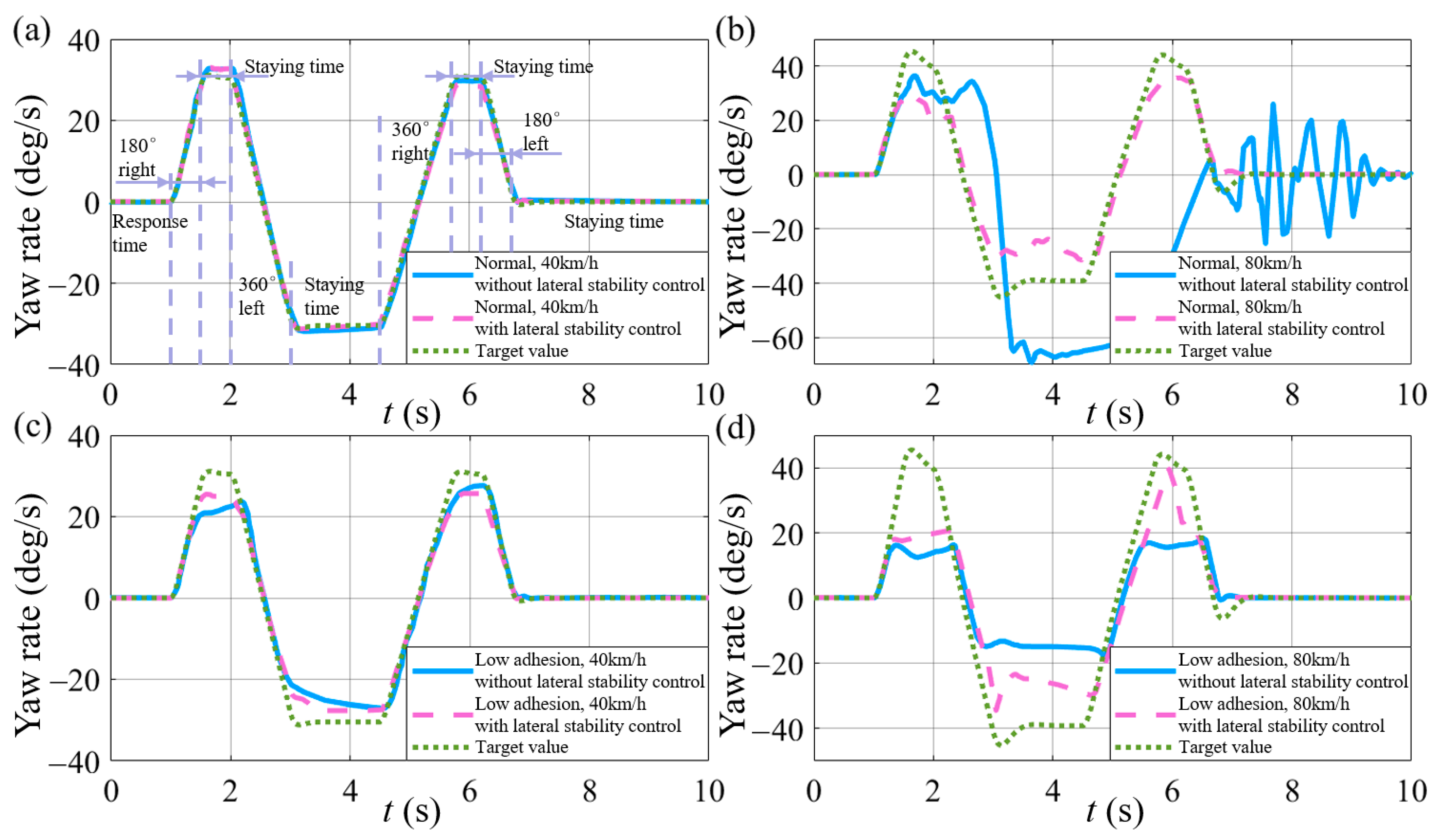
The simulation results of the PID algorithm show that the yaw rate curves at the different road conditions and speed conditions were corrected to a certain extent, which verified that the algorithm can be effectively adapted to the different road conditions and vehicle speeds.
(2)
The simulation results without iterative training show that the yaw rate curve is smoother. And the fluctuation of the curve was corrected as the training was iterated. The algorithm can prevent the accident from sudden changes and optimize itself continuously.
(3)
The training results of the BP neural network-based PID algorithm show that the correction effect of this algorithm for yaw rate was further improved, which improves the stability of the BP neural network-based PID algorithm by improving the responsive speed.
The above results show that the algorithm was proved to be effective. The algorithm can automatically adjust the control parameters and automatically optimize the control process following the feedback from the controlled system, which allows it to adapt to more road situations and environments and provides a feasible idea for the development of a more intelligent and general automotive electronic stabilization system.

Author Contributions

Conceptualization, Z.W.; methodology, Z.W.; software, Z.W.; validation, Z.W. and B.L.; formal analysis, Z.W. and X.Z.; investigation, Z.W. and B.L.; resources, Z.W. and X.Z.; data curation, C.K.; writing-original draft preparation, Z.W.; writing-review and editing, J.R.; visualization, J.R.; supervision, C.K.; project administration, C.K.; funding acquisition, C.K. All authors have read and agreed to the published version of the manuscript.

Funding

This research was funded by Robot and high-end equipment government funds grant number [No. 2022Z073]. The APC was funded by Jiageng Ruan.

Data Availability Statement

The data presented in this study are available on request from the corresponding author. The data are not publicly available due to the policy for cooperating enterprises.

Conflicts of Interest

The authors declare no conflicts of interest.

References

  1. Kim, D.; Kim, K.; Lee, W.; Hwang, I. Development of Mando ESP (Electronic Stability Program); Report no. 0148-7191; SAE Technical Paper; SAE International: Warrendale, PA, USA, 2003. [Google Scholar]
  2. Liu, K.; Gong, J.; Kurt, A.; Chen, H.; Ozguner, U. Dynamic Modeling and Control of High-Speed Automated Vehicles for Lane Change Maneuver. IEEE Trans. Intell. Veh. 2018, 3, 329–339. [Google Scholar] [CrossRef]
  3. González, D.; Pérez, J.; Milanés, V.; Nashashibi, F. A Review of Motion Planning Techniques for Automated Vehicles. IEEE Trans. Intell. Transp. Syst. 2016, 17, 1135–1145. [Google Scholar] [CrossRef]
  4. Ju, Z.; Zhang, H.; Li, X.; Chen, X.; Han, J.; Yang, M. A Survey on Attack Detection and Resilience for Connected and Automated Vehicles: From Vehicle Dynamics and Control Perspective. IEEE Trans. Intell. Veh. 2022, 7, 815–837. [Google Scholar] [CrossRef]
  5. Schwarting, W.; Alonso-Mora, J.; Pauli, L.; Karaman, S.; Rus, D. Parallel autonomy in automated vehicles: Safe motion generation with minimal intervention. In Proceedings of the 2017 IEEE International Conference on Robotics and Automation (ICRA), Singapore, 29 May–3 June 2017; pp. 1928–1935. [Google Scholar]
  6. Cheng, S.; Wang, Z.; Yang, B.; Li, L.; Nakano, K. Quantitative Evaluation Methodology for Chassis-Domain Dynamics Performance of Automated Vehicles. IEEE Trans. Cybern. 2022, 53, 5938–5948. [Google Scholar] [CrossRef]
  7. Li, X. Trade-off between safety, mobility and stability in automated vehicle following control: An analytical method. Transp. Res. Part B Methodol. 2022, 166, 1–18. [Google Scholar] [CrossRef]
  8. Kang, C.; Shi, C.; Liu, Z.; Liu, Z.; Jiang, X.; Chen, S.; Ma, C. Research on the optimization of welding parameters in high-frequency induction welding pipeline. J. Manuf. Process. 2020, 59, 772–790. [Google Scholar] [CrossRef]
  9. Wang, P.; Pang, H.; Xu, Z.; Jin, J. Co-Estimation and Validation of Driving States of a 3-DOFs Vehicle Model Based on UKF Approach. In Proceedings of the 2021 33rd Chinese Control and Decision Conference (CCDC), Kunming, China, 22–24 May 2021; IEEE: Piscataway, NJ, USA, 2021; pp. 6504–6510. [Google Scholar]
  10. Li, G.; Hong, W.; Zhang, D.; Zong, C. Research on control strategy of two independent rear wheels drive electric vehicle. Phys. Procedia 2012, 24, 87–93. [Google Scholar] [CrossRef]
  11. Fu, Q.; Zhao, L.; Cai, M.; Cheng, M.; Sun, X. Simulation research for quarter vehicle ABS on complex surface based on PID control. In Proceedings of the 2012 2nd International Conference on Consumer Electronics, Communications and Networks (CECNet), Yichang, China, 21–23 April 2012; pp. 2072–2075. [Google Scholar]
  12. Cao, J.; Song, C.; Peng, S.; Song, S.; Zhang, X.; Xiao, F. Trajectory tracking control algorithm for autonomous vehicle considering cornering characteristics. IEEE Access 2020, 8, 59470–59484. [Google Scholar] [CrossRef]
  13. Dong, X.; Li, L.; Cheng, S.; Wang, Z. Integrated strategy for vehicle dynamics stability considering the uncertainties of side-slip angle. IET Intell. Transp. Syst. 2020, 14, 1116–1124. [Google Scholar] [CrossRef]
  14. Peng, Z.; Ning, G. 2 DOF lateral dynamic model with force input of skid steering wheeled vehicle. In Proceedings of the 2014 IEEE Conference and Expo Transportation Electrification Asia-Pacific (ITEC Asia-Pacific), Beijing, China, 31 August–3 September 2014; IEEE: Piscataway, NJ, USA, 2014; pp. 1–5. [Google Scholar]
  15. Chu, L.; Gao, X.; Guo, J.; Liu, H.; Chao, L.; Shang, M. Coordinated control of electronic stability program and active front steering. Procedia Environ. Sci. 2012, 12, 1379–1386. [Google Scholar] [CrossRef]
  16. Tekin, G.; Samim Unlusoy, Y. Design and simulation of an integrated active yaw control system for road vehicles. Int. J. Veh. Des. 2009, 52, 5–19. [Google Scholar] [CrossRef]
  17. Ni, J.; Hu, J. Handling performance control for hybrid 8-wheel-drive vehicle and simulation verification. Veh. Syst. Dyn. 2016, 54, 1098–1119. [Google Scholar] [CrossRef]
  18. Wang, H.; Xue, C. Modelling and Simulation of Electric Stability Program for the Passenger Car; Report no. 0148-7191; SAE Technical Paper; SAE International: Warrendale, PA, USA, 2004. [Google Scholar]
  19. Sabbioni, E.; Cheli, F. Analysis of ABS/ESP Control Logics Using a HIL Test Bench; Report no. 0148-7191; SAE Technical Paper; SAE International: Warrendale, PA, USA, 2011. [Google Scholar]
  20. Yu, H.; Cheli, F.; Castelli-Dezza, F. Optimal design and control of 4-IWD electric vehicles based on a 14-DOF vehicle model. IEEE Trans. Veh. Technol. 2018, 67, 10457–10469. [Google Scholar] [CrossRef]
  21. Perrelli, M.; Cosco, F.; Carbone, G.; Mundo, D. Evaluation of vehicle lateral dynamic behaviour according to ISO-4138 tests by implementing a 15-DOF vehicle model and an autonomous virtual driver. Int. J. Mech. Control 2019, 20, 31–38. [Google Scholar]
  22. Lu, X.; Shi, Q.; Li, Y.; Xu, K.; Tan, G. Road Adhesion Coefficient Identification Method Based on Vehicle Dynamics Model and Multi-Algorithm Fusion; Report no. 0148-7191; SAE Technical Paper; SAE International: Warrendale, PA, USA, 2022. [Google Scholar]
  23. Zhang, X.; Xu, Y.; Pan, M.; Ren, F. A vehicle ABS adaptive sliding-mode control algorithm based on the vehicle velocity estimation and tyre/road friction coefficient estimations. Veh. Syst. Dyn. 2014, 52, 475–503. [Google Scholar] [CrossRef]
  24. Savitski, D.; Schleinin, D.; Ivanov, V.; Augsburg, K.; Jimenez, E.; He, R.; Sandu, C.; Barber, P. Improvement of traction performance and off-road mobility for a vehicle with four individual electric motors: Driving over icy road. J. Terramech. 2017, 69, 33–43. [Google Scholar] [CrossRef]
  25. Yuan, C.-c.; Chen, L.; Wang, S.-h.; Jiang, H.-b. Research of electronic stability program based on the Mu control theory. In Proceedings of the 2010 International Conference on Computer and Communication Technologies in Agriculture Engineering, Chengdu, China, 12–13 June 2010; IEEE: Piscataway, NJ, USA, 2010; pp. 379–381. [Google Scholar]
  26. Bo, L.; Cheng, Y.H. Robust controller design for regenerative braking control of electric vehicles. In Proceedings of the 2011 6th IEEE Conference on Industrial Electronics and Applications, Beijing, China, 21–23 June 2011; pp. 214–219. [Google Scholar]
  27. Zhang, J.; Wang, H.; Zheng, J.; Cao, Z.; Man, Z.; Yu, M.; Chen, L. Adaptive sliding mode-based lateral stability control of steer-by-wire vehicles with experimental validations. IEEE Trans. Veh. Technol. 2020, 69, 9589–9600. [Google Scholar] [CrossRef]
  28. Jin, L.; Xie, X.; Shen, C.; Wang, F.; Wang, F.; Ji, S.; Guan, X.; Xu, J. Study on electronic stability program control strategy based on the fuzzy logical and genetic optimization method. Adv. Mech. Eng. 2017, 9, 1687814017699351. [Google Scholar] [CrossRef]
  29. Jin, L.-q.; Song, C.-x.; Li, J.-h. Controll algorithm of combination with logic gate and PID control for vehicle electronic stability control. In Proceedings of the 2010 2nd International Conference on Advanced Computer Control, Shenyang, China, 27–29 March 2010; IEEE: Piscataway, NJ, USA, 2010; pp. 345–349. [Google Scholar]
  30. Taghavifar, H.; Hu, C.; Taghavifar, L.; Qin, Y.; Na, J.; Wei, C. Optimal robust control of vehicle lateral stability using damped least-square backpropagation training of neural networks. Neurocomputing 2020, 384, 256–267. [Google Scholar] [CrossRef]
  31. Li, C.; He, C.; Yuan, Y.; Zhang, J. Yaw stability control based on a novel electronic hydraulic braking system. In Proceedings of the 2019 IEEE 8th Joint International Information Technology and Artificial Intelligence Conference (ITAIC), Chongqing, China, 24–26 May 2019; IEEE: Piscataway, NJ, USA, 2019; pp. 1395–1399. [Google Scholar]
  32. Yu, C.-H.; Tseng, C.-Y.; Hsu, Y.-S. Electronic stability control for direct-drive Electric Vehicle. In Proceedings of the 2011 International Conference on Electric Information and Control Engineering, Wuhan, China, 15–17 April 2011; IEEE: Piscataway, NJ, USA, 2011; pp. 4987–4991. [Google Scholar]
  33. Wang, J.; Qiao, J.; Qi, Z. Research on control strategy of regenerative braking and anti-lock braking system for electric vehicle. In Proceedings of the 2013 World Electric Vehicle Symposium and Exhibition (EVS27), Barcelona, Spain, 17–20 November 2013; pp. 1–7. [Google Scholar]
  34. Drakunov, S.; Ozguner, U.; Dix, P.; Ashrafi, B. ABS control using optimum search via sliding modes. IEEE Trans. Control Syst. Technol. 1995, 3, 79–85. [Google Scholar] [CrossRef]
  35. Li, Z.; Wang, P.; Liu, H.; Hu, Y.; Chen, H. Coordinated longitudinal and lateral vehicle stability control based on the combined-slip tire model in the MPC framework. Mech. Syst. Signal Process. 2021, 161, 107947. [Google Scholar] [CrossRef]
  36. Cho, K.; Kim, J.; Choi, S. The integrated vehicle longitudinal control system for ABS and TCS. In Proceedings of the 2012 IEEE International Conference on Control Applications, Dubrovnik, Croatia, 3–5 October 2012; pp. 1322–1327. [Google Scholar]
  37. Guo, J.; Chu, L.; Liu, H.; Shang, M.; Fang, Y. Integrated control of active front steering and electronic stability program. In Proceedings of the 2010 2nd International Conference on Advanced Computer Control, Shenyang, China, 27–29 March 2010; IEEE: Piscataway, NJ, USA, 2010; pp. 449–453. [Google Scholar]
  38. Tian, Y.; Cao, X.; Wang, X.; Zhao, Y. Four wheel independent drive electric vehicle lateral stability control strategy. IEEE/CAA J. Autom. Sin. 2020, 7, 1542–1554. [Google Scholar] [CrossRef]
  39. Fittro, R.; Knospe, C. μ Control of a High Speed Spindle Thrust Magnetic Bearing. In Proceedings of the 1999 IEEE International Conference on Control Applications (Cat. No.99CH36328), IEEE, Kohala Coast, HI, USA, 22–27 August 1999; Volume 1, pp. 570–575. [Google Scholar]
  40. Setiawan, J.D.; Safarudin, M.; Singh, A. Modeling, simulation and validation of 14 DOF full vehicle model. In Proceedings of the International Conference on Instrumentation, Communication, Information Technology, and Biomedical Engineering 2009, Bandung, Indonesia, 23–25 November 2009; pp. 1–6. [Google Scholar]
  41. Shim, T.; Ghike, C. Understanding the limitations of different vehicle models for roll dynamics studies. Veh. Syst. Dyn. 2007, 45, 191–216. [Google Scholar] [CrossRef]
  42. Pacejka, H. Modelling of the Pneumatic Tyre and Its Impact on Vehicle Dynamic Behaviour; Vehicle Research Laboratory, Delft University of Technology: Delft, The Netherlands, 1989. [Google Scholar]
  43. Svoboda, M.; Biba, D.; Musuroi, S.; Ancuti, C.-M.; Sorandaru, C. Modeling of squirrel cage induction machine with S-function in MATLAB Simulink. In Proceedings of the 2017 14th International Conference on Engineering of Modern Electric Systems (EMES), Oradea, Romania, 1–2 June 2017; IEEE: Piscataway, NJ, USA, 2017; pp. 176–179. [Google Scholar]
  44. Ivanov, V. A review of fuzzy methods in automotive engineering applications. Eur. Transp. Res. Rev. 2015, 7, 29. [Google Scholar] [CrossRef]
Figure 1. The composition of the automotive electronic stability system electronic control unit.
Actuators 13 00100 g001
Figure 2. 2-DOF model of vehicle.
Actuators 13 00100 g002
Figure 3. Schematic diagram of the motion of the center of mass.
Actuators 13 00100 g003
Figure 4. Predictive model of a vehicle with 2-DOF.
Actuators 13 00100 g004
Figure 5. Pitch motion and lateral motion model.
Actuators 13 00100 g005
Figure 6. Suspension model of a vehicle with 7 DOF.
Actuators 13 00100 g006
Figure 7. Manipulation model of a vehicle with 7-DOF.
Actuators 13 00100 g007
Figure 8. Simulation model of a vehicle with a 14-DOF model.
Actuators 13 00100 g008
Figure 9. Yaw rates for the predictive model and the simulation model.
Actuators 13 00100 g009
Figure 10. (a) Imported CarSim real-time correlation model of the vehicle. (b) Simulation model of the lateral electronic stability controller.
Actuators 13 00100 g010
Figure 11. BP neural network PID controller workflow.
Actuators 13 00100 g011
Figure 12. Comparison of the yaw rate profile at an initial speed of (a) 40 km/h on a normal road; (b) 80 km/h on normal roads; (c) 40 km/h on a low adhesion road; and (d) 80 km/h on a low adhesion road.
Actuators 13 00100 g012
Figure 13. Comparison of yaw rate curve of target values, with and without lateral stability control.
Actuators 13 00100 g013
Figure 14. Comparison of 14-DOF model with CarSim simulation model.
Actuators 13 00100 g014
Figure 15. Comparison of yaw rate curve of target values, initial state, after 100 iterations of training, after 1000 iterations of training, and fuzzy controller.
Actuators 13 00100 g015
Table 1. Hyperparameters in the magic formula for tire.
FxFyMz
Xobtained from S in Equation (17)obtained from α in Equation (14)obtained from α in Equation (14)
Dobtained from Fz in Equation (9)obtained from Fz in Equation (9)obtained from Fz in Equation (9)
C1.651.302.40
Bobtained from Fz, C, and Dobtained from Fz, C, and Dobtained from Fz, C, and D
Eobtained from Fz in Equation (9)obtained from Fz in Equation (9)obtained from Fz in Equation (9)
Disclaimer/Publisher’s Note: The statements, opinions and data contained in all publications are solely those of the individual author(s) and contributor(s) and not of MDPI and/or the editor(s). MDPI and/or the editor(s) disclaim responsibility for any injury to people or property resulting from any ideas, methods, instructions or products referred to in the content.

